Thesis
Profiling the turbulent atmosphere and novel correction techniques for imaging and photometry in astronomy
James Osborn
A Thesis presented for the degree of
Doctor of Philosophy

Centre for Advanced Instrumentation
Department of Physics
Durham University
England
August 2010
Submitted for the degree of Doctor of Philosophy
August 2010
Abstract
The turbulent atmosphere has two detrimental effects in astronomy. The phase aberration induced by the turbulence broaden the point spread function (PSF) and limits the resolution for imaging. If there is strong turbulence high in the atmosphere then these phase aberration propagate and develop into intensity fluctuations (scintillation). This thesis describes three novel instruments related to these problems associated with atmospheric turbulence. The first is an optical turbulence profiler to measure the turbulence strength and its position within the atmospheric surface layer in real-time. The instrument is a development of the slope detection and ranging (SLODAR) method. Results from the prototype at Paranal Observatory are discussed. An instrument to improve the PSF for imaging is also discussed. The instrument works by adaptively blocking the telescope pupil to remove areas which are the most out of phase from the mean. This acts to flatten the wavefront and can therefore be used after an adaptive optics system as an additional clean up, or stand alone on a telescope as a relatively affordable and easy way to improve the PSF. The third instrument reduces the scintillation noise for high precision fast photometry. Simulation results show that it is possible to reduce the scintillation noise to a level where the measurements are photon noise dominated.
Declaration
The work in this thesis is based on research carried out at the Centre for Advanced Instrumentation, the Department of Physics, University of Durham, England. No part of this thesis has been submitted elsewhere for any other degree or qualification and it is the sole work of the author unless referenced to the contrary in the text.
Some of the work presented in this thesis has been published in journals – the relevant publications are listed below.
Publications
James Osborn, R. W. Wilson, V. Dhillon, R. Avila, and G. D. Love. High precision fast photometry from ground based observatories. MNRAS, submitted 17/08/2010.
James Osborn, R. W. Wilson, T. Butterley, H. Shepherd, and M. Sarazin. Profiling the surface layer of optical turbulence with slodar. MNRAS, 406(2), 1405–1408, 2010.
James Osborn, Richard M. Myers, and Gordon D. Love. Reducing PSF halo with adaptive pupil masking. SPIE, 7736–102, in press, 2010
G. Lombardi, J. Melnick, R. H. Hinojosa Goi, J. Navarrete, M. Sarazin, A. Berdja, A. Tokovinin, R. Wilson, J. Osborn, T. Butterley and H. Shepherd. Surface Layer characterisation at Paranal Observatory. SPIE, 7733–159, in press, 2010
James Osborn, Richard M. Myers, and Gordon D. Love. PSF halo reduction in adaptive optics using dynamic pupil masking. Optics Express, 17(20):17279–17292, 2009.
James Osborn, R. W. Wilson, and T. Butterley. Surface layer SLODAR. In E. Masciadri and M. Sarazin, editors, Optical Turbulence: Astronomy meets Meteorology, pages 371–378, 2008.
R. W. Wilson, T. Butterley and James Osborn. SLODAR turbulence monitors. In E. Masciadri and M. Sarazin, editors, Optical Turbulence: Astronomy meets Meteorology, pages 50–57, 2008.
Copyright Ⓒ 2010 by James Osborn.
“The copyright of this thesis rests with the author. Information derived from it should be acknowledged”.
Acknowledgements
I would like to thank all my friends and family for all of their support during the last four years. I would like to especially thank Clare for sticking with it and trying to be interested in all of the rubbish I have to say at the end of the day.
I would like to thank my supervisor, Gordon Love, for keeping me on track and coming up with some great ideas. I would also like to thank my unofficial supervisor, Richard Wilson, for all his help despite getting no teaching credits for it. In addition I would like to thank everyone who has collaborated with me and helped to develop the ideas presented here, in particular the SLODAR team deserve a special mention. All past and present occupants of 125b whose tenancies overlapped with myself, including Luke Tyas, Claire Poppett, Mark Harrison, Jonny Taylor, Tim Butterley and Chris Saunter. Luke and Claire always provide a worthwhile distraction. I thank Mark for his help in trying to decipher the sometimes twisted logic of the old AO simulation, Jonny for his logical input on all matters, Tim and Chris for getting me started right at the beginning, always being there to answer those awkward questions and frequent distractions throughout. I would also like to mention the self professed ‘gatekeeper of science’, Tim Morris, for all his helpful rants and chats, usually down the pub.
List of Figures
1.1 Example simulated images for a diffraction limited system and a turbulence limited system
2.1 Example Kolmogorov phase aberrations
2.2 Example non–Kolmogorov phase aberrations
2.3 Example power spectra for Kolmogorov and non–Kolmogorov turbulence.
2.4 Example simulated images for a diffraction limited system and a turbulence limited system
2.5 Example simulated long exposure images for a diffraction limited system and a turbulence limited system
2.6 Telescope and atmospheric MTF
2.7 Simple diagram of AO system.
2.8 Diagram of a Shack–Hartmann wavefront sensor
2.9 Theoretical plots to show the effect of an AO system on the wavefront structure function
2.10 Atmospheric modulation transfer function after AO correction.
2.11 Scintillated pupil image.
2.12 Example pupil images for no turbulence (a) and a turbulent layer at 1 km (b), 5 km (c) and 10 km (d).
2.13 Scintillation pattern spatial covariance functions.
2.14 Scintillation modified phase power spectrum.
2.15 Diagram of the LuSci geometry.
2.16 Diagram of the triangulation method for turbulence profiling.
2.17 SLODAR geometry
2.18 Example 2D auto-covariance and cross-covariance maps.
2.19 SLODAR 1D cross-covariance
2.20 SLODAR impulse response functions in the longitudinal and transverse directions
2.21 Example SLODAR profile
2.22 Example 2D auto-covariance and cross-covariance maps with temporal offset.
3.1 Diagram of the SL–SLODAR instrument.
3.2 Example average SH spot pattern from a single camera
3.3 Time averaged centroid variance for the single camera wavefront sensor
3.4 SL–SLODAR beam splitter
3.5 Diagram of SLODAR optics and dimensions
3.6 Photograph of the SL–SLODAR identifying the optical components.
3.7 Photograph of the SL–SLODAR on the 16 inch Meade telescope at Paranal.
3.8 Example SH spot patterns from two cameras
3.9 Time averaged centroid variance for two cameras.
3.10 Example SL–SLODAR profile sequence for the night of 9th April 2009
3.11 Vertical resolution histogram.
3.12 SLODAR median surface layer profile for data acquired on 17 nights in February 2009 and April 2009, at Cerro Paranal, Chile
3.13 SL–SLODAR and DIMM seeing comparison
3.14 SL–SLODAR and DIMM Cn2 comparison
3.15 Comparison of the integrated turbulence strength for the surface layer between SL–SLODAR and MASS–DIMM.
3.16 Comparison of the integrated turbulence strength for the surface layer as measured by SL–SLODAR and LuSci
3.17 Comparison of the integrated turbulence strength for the surface layer as measured by LuSci and DIMM – MASS
3.18 SL–SLODAR profile from 08/04/2009
3.19 SL–SLODAR profile from 10/02/2009
3.20 MASS profile from 10/02/2009
3.21 SL–SLODAR profile from 13/02/2009
4.1 Block diagram for the adaptive pupil mask system.
4.2 Simulation results showing how the FWHM of the PSF is modified by the adaptive pupil mask.
4.3 Simulation results showing how the peak intensity of the PSF is modified by the adaptive pupil mask.
4.4 Example PSF from a 1 m telescope without AO with r0 = 0.15 m.
4.5 Example PSF from an 8 m telescope equipped with a 16×16 AO system with r0 = 0.15 m.
4.6 SNR obtained as a function of threshold for observing a faint companion at 2λ∕D.
4.7 Radial cut through of coronagraph PSF
4.8 APM performance comparing residual variance and mean pupil fraction blocked.
4.9 Atmospheric modulation transfer function after AO correction.
4.10 Atmospheric modulation transfer function without AO correction.
4.11 Masked telescope transfer function
4.12 2D telescope modulation transfer plot.
4.13 Diffraction limited PSFs for blocked pupil fractions of 0.0, 0.2, 0.4 and 0.6.
4.14 Diffraction limited PSFs for blocked pupil fractions of 0.0, 0.2, 0.4 and 0.6, log10 plot.
4.15 Combined MTF from the telescope and atmosphere, MTFatmos×MTFtel.
4.16 Theoretical PSF after pupil masking
5.1 Conceptual design for one arm of the instrument.
5.2 Prototype of the conjugate-plane photometer.
5.3 Scintillation diagram.
5.4 Reducing scintillation with an aperture in the sky.
5.5 Ray diagrams for conjugation positions.
5.6 Re-conjugated pupil intensity images for a number of aperture diameters and increasing propagation distance.
5.7 Diagrams of light cones for differential photometry.
5.8 Simulated pupil intensity patterns at the telescope pupil and at the conjugate altitude of the turbulent layer.
5.9 Pupil images conjugate to 10 km for two stars separated by 40′′.
5.10 Scintillation variance as a function of aperture size.
5.11 Example simulated light curves for the normal and reconjugated pupils.
5.12 An example simulated light curve.
5.13 Instrument sensitivity to the conjugate altitude.
5.14 Instrument sensitivity to additional turbulent layers at intermediate altitudes.
5.15 Comparison of simulated and predicted corrected scintillation variance.
5.16 SCIDAR turbulence profile from 19th May 2000 at San Pedro M´artir.
5.17 Predicted improvement in intensity variance as a function of time for the night of 19th May 2000.
5.18 Predicted scintillation variance as a function of time for the night of 19th May 2000.
5.19 Simulated light curve of a secondary transit of an extrasolar planet with and without scintillation reduction
5.20 Predicted improvement ratios for varying target magnitudes and telescope sizes.
Chapter 1
Introduction
1.1 Motivation
1.2 Synopsis
1.1 Motivation
Throughout history humans have turned their attention to the skies and questioned our position within the universe. Only recently has it been possible through the development of sophisticated observational techniques and instrumentation to confirm the existence of other planets orbiting the stars in our galaxy. At the date of writing this (August 2010) there are nearly 500 confirmed extrasolar planet detections. A variety of methods have been used to find these planets each one favouring planets of a certain mass range at a certain distance from the host star. All of the techniques, except direct imaging of the planet, involves inferring its presence by its effect on the star or the light from the star. Direct imaging of an extrasolar planet is very exciting as it allows spectroscopic and photometric characterisation of the planets atmosphere, which is of great interest for planetary formation and evolution studies [1, 2, 3]. However, direct imaging is a challenge due to the brightness difference and the small angular separations of the star / planet system as viewed from the Earth. So far only very large planets orbiting at large separations have been directly observed but this mile stone observation is leading the way to the ‘holy grail’ of extrasolar planet detection which is to detect an Earth sized planet in the habitable zone as these are the only ones which are thought to be capable of supporting life [4]. Currently the only detection technique with the sensitivity required to potentially detect an Earth sized planet in a realistic time frame is the transit method [5]. As the planet passes between us and the star it obscures a small area of the star, blocking some of its light. This reduction in intensity can be measured and used to infer not only the presence of the planet but a wealth of information about it. Examining the transit curve can provide us with the planets radius, temperature, albedo, atmospheric dynamics and composition and when combined with measurements of the radial velocity, which are required anyway to remove false positives, the planetary mass, density and hence its composition can also be estimated [6].
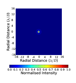
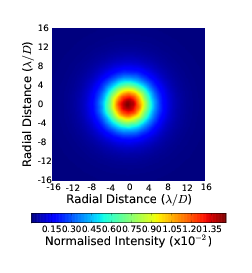
Ground based observatories are favourable to space based as they can be made much larger, are cheaper per unit area of telescope and are easier to maintain and upgrade. Space based instruments are expensive and complicated. However, often a lot of money is spent on sending telescopes into space. This is because of the Earth’s atmosphere. In some spectral bands observations form the ground are impossible due to the atmospheric absorption. In other bands the transmission is high but the atmospheric turbulence significantly degrades the image. Figure 1.1 shows a simulated example of a short exposure image of a diffraction limited system (i.e. no turbulence, the image size is determined by the size and quality of the telescope and its optics) and an image through strong turbulence. It is obvious that it would be much easier to distinguish two objects which are close together in the diffraction limited image.
 |  |
| (a) | (b) |
Figure 1.1: Example simulated long exposure images through a diffraction limited system (a) and an image through strong turbulence (b). The light is spread over a much larger area making high resolution and high contrast imaging very difficult. The intensity is normalised to the peak intensity of the diffraction limited case.
The Earth’s atmosphere is a shell of gasses surrounding the planet that is retained by gravity. It is impossible to define a point where the atmosphere ends and outer space begins but it is generally accepted (by the Fédération Aéronautique Internationale) to be at the Kármán line at 100 km. However, about three quarters of the total mass of the atmosphere is located within the first ~12 km from the ground. This boundary is called the tropopause and is the point where the air no longer cools with increasing altitude and is essentially void of water vapour. Although turbulent air flow can occur above the tropopause the lack of water vapour means that there is very little in the way of weather systems present at altitude. Optical turbulence or ‘clear air turbulence’ as it is known by meteorologists is different from the large scale turbulence which gives rise to weather systems. Optical turbulence is caused by the mechanical mixing of layers of air with different temperatures and hence density. As the refractive index of air changes with density this turbulence creates a continuous screen of spatially and temporally varying refractive indices. Above the tropopause the temperature of the air is constant with altitude resulting in very little high altitude optical turbulence. In the troposphere there is a very steep temperature gradient creating conditions perfect for optical turbulence. The optical turbulence profile (turbulence strength as a function of altitude) changes with location and time. However, luckily for astronomers, we do not observe a volume of optical turbulence in this zone but several thin discrete layers [7]. In general premiere observing sites will include a strong turbulent layer at the ground generated by solar heating during the day and surface winds perturbed by objects. There is also usually a strong turbulent layer at the tropopause caused by wind shear between two layers in the atmosphere [8]. Often thin turbulent layers are also observed at altitudes between these layers but rarely above.
In the case of optical imaging, high resolution and high contrast imaging is made possible form the Earth’s surface with adaptive optics (AO) systems. AO uses a wavefront sensor to measure the phase aberrations and a deformable mirror to flatten the wavefront. The purpose of which is to focus all of the star light into a well defined diffraction limited point. Without this the light would smear out into a large (in spatial extent) halo. This halo will make imaging of faint companions very difficult (see figure 1.1). AO is now capable of very good correction over a very small field of view, ideal for the imaging of extrasolar planets. With new advances in AO concepts and technology it is also now possible to obtain good correction over a large field of view. However, no AO system is perfect and there are always residual wavefront errors. The technology is still very much in development and there is room for improvement. These improvements are made by using new understanding of the atmosphere and its behaviour to generate new ideas. Corrective imaging techniques are in an era of massive development.
The atmosphere also perturbs the intensity of the image, this can be observed by the naked eye as twinkling or scintillation. The scintillation limits the precision of possible photometric measurements. However, unlike AO for imaging there is currently no instrumentation dedicated to reducing scintillation. There are some ‘tricks of the trade’, for example increasing the exposure time or simply using a larger telescope to temporally or spatially average over the intensity fluctuations. However, it is not always possible or practical to use time on larger telescopes for photometric studies and this will be limited to very faint targets and short exposure times to avoid saturation and may still be limited by scintillation. Time averaging the intensity (i.e. increasing the exposure time) will reduce the scintillation noise. However, for fast photometry, time averaging can also only be used in circumstances where the target intensity fluctuations have a much longer time scale than the scintillation. This may not be the case if you want to make several measurements across a transit of an hour or so, as would be the case for an Earth like planet.
In order to develop ideas for new imaging and scintillation correction techniques we must first understand the structure and behaviour of the atmosphere. This can be done by examining data from turbulence profiling instruments (e.g. SLOpe Detection And Ranging, SLODAR [9], or SCItillation Detection And Ranging, SCIDAR [10]). This information is also required to model and optimise modern sophisticated AO systems which correct each individual turbulent layer independently in order to increase the homogeneously corrected field of view and for observatory site selection and characterisation. For these last two applications the surface layer is particularly important. Studies show [7, 11, 12, 13] that at many observatories this surface layer tends to be very thin and contain a large fraction of the turbulence.
1.2 Synopsis
In chapter 2 we discuss the relevant theory required for the concepts discussed in the later chapters. None of the material in this chapter is original work.
In chapter 3 we discuss a modification to the SLODAR instrument to profile specifically the surface layer of optical turbulence, named surface layer SLODAR or SL–SLODAR. Previous studies using SLODAR have shown that the surface layer at Paranal observatory is very thin [7]. It was unresolved with vertical resolutions of ~100 m. SLODAR functions by triangulating the altitude of the turbulent layer by comparing the wavefronts from two target stars. The altitude resolution of SLODAR is governed by the instrument optics and the target stars angular separation. By increasing this angular separation we can increase the altitude resolution. SL–SLODAR works by separating the light from the two stars into separate cameras allowing for much wider separations and consequently much higher altitude resolution. By targeting stars with an angular separation of approximately 16 arcminutes we can obtain resolutions of ~10 m.
In chapter 4 we examine an idea to reduce the wavefront phase variance for high contrast imaging. The concept involves using an adaptive pupil mask to block areas of the telescope pupil which are out of phase with the mean wavefront position. By doing this we actively flatten the wavefront and reduce areas of the wavefront from constructively interfering and generating speckles which average in long exposures to form the PSF halo. The instrument could be used either after an AO system to further improve the image quality or on a telescope without AO as a relatively easy and cheap form of image correction.
In chapter 5 we present a passive technique to reduce the atmospheric effects on the intensity of a stars image. In a similar way that AO has allowed imaging of extrasolar planets from the Earth’s surface it is hoped that this method will allow high precision photometry from the Earth’s surface and potentially lead to the routine characterisation of extrasolar planets from the ground.
Finally, Chapter 6 summarises the conclusions drawn from this work and describes the future prospects for the projects.
Chapter 2
Theory
2.1 Atmospheric Turbulence
2.1.1 Kolmogorov atmospheric turbulence
2.1.2 Non Kolmogorov atmospheric turbulence
2.1.3 Inner and Outer Scale
2.2 Imaging through turbulence
2.3 Adaptive Optics
2.3.1 Wavefront sensing
2.3.2 Imaging with Adaptive optics
2.3.3 AO Taxonomy
2.4 Photometry through atmospheric turbulence
2.4.1 Scintillation
2.5 Numerical Simulations
2.5.1 AO simulations
2.5.2 Fresnel Simulations
2.6 Site Characterisation
2.7 Turbulence Monitoring Instrumentation
2.7.1 Differential Image Motion Monitor (DIMM)
2.7.2 Multi-Aperture Scintillation Sensor (MASS)
2.7.3 Lunar Scintillometer (LuSci)
2.7.4 SCIntillation Detection And Ranging (SCIDAR)
2.8 SLOpe Detection And Ranging (SLODAR)
2.8.1 SLODAR data analysis
2.1 Atmospheric Turbulence
The wavefront from an astronomical source can be considered flat at the top of the atmosphere. As it propagates to the ground it gets corrupted by the optical turbulence which forms a limit to the precision of measurements from ground based telescopes. Optical turbulence is caused by the mechanical mixing of layers of air with different temperatures and hence density. As the refractive index of air changes with density this turbulence creates a continuous screen of spatially and temporally varying refractive indices. Although each of the refractive index inhomogeneities in the turbulent layers may be small the wavefront passes through a large number of them and the cumulative effect can be quite large. The cumulative refractive index variations delay parts of the incoming wavefront with respect to others. The net effect is that the wavefront becomes aberrated. If we assume a horizontal turbulent layer at altitude, h, above the ground and that the layer thickness, δh, is large compared to the eddy size of the refractive index inhomogeneites but small enough so that we can ignore diffraction effects within the layer (thin screen approximation [14]) then the phase fluctuations, ϕ(ε), induced by the turbulent layer is related to the refractive index fluctuations, n(h,ε), along the propagation path by
 | (2.1) |
where k is the wave number, 2π∕λ, with λ being the wavelength of the light and ε is a spatial parameter. The wavefunction after the layer is then,
 | (2.2) |
It is these aberrations in the wavefront which act to distort images from astronomical telescopes. We are therefore not interested in the absolute value of the phase only the difference between its value at two points, which is caused by the spatial variance of the refractive index. The refractive index structure function, Dn(ρ), is the spatial variance in the difference of refractive index as a function of separation [15],
 | (2.3) |
where ⟨⟩ denotes an ensemble average, Dn(ρ) depends only on the difference in refractive index with separation, ρ, and not the position, ε. Cn2(h) is the refractive index structure constant and is therefore a measure of the amount of local refractive index inhomogeneites and can be used to quantify the strength of the optical turbulence. The units of Cn2(h) is m-2∕3. The turbulent layers do have a finite thickness so it is usually more useful to look at the integrated refractive index structure constant, ∫ h1h2Cn2(h)dh, between two altitude limits which tells us the integrated turbulence strength of the optical turbulence in that range with units of m1∕3.
The Fried parameter is often used to quantify the integrated strength of the turbulence. This is a useful parameter as it is defined as the diameter of an aperture in which the phase variance, σϕ2 is approximately one. Stronger turbulence will therefore correspond to a smaller r0. r0 is related to Cn2(h) by [14],
 | (2.4) |
where γ is the zenith angle.
2.1.1 Kolmogorov atmospheric turbulence
Turbulent flow is very complicated and still not entirely understood. Andrei Kolmogorov developed a simple physical model for turbulence that could be used to analytically evaluate its effects. Kolmogorov’s model assumes that energy is injected into the turbulent medium on large spatial scales (the outer scale, L0) and forms eddies. These then break down into smaller eddies in a self-similar cascade until the eddies become small enough that the energy is dissipated by the viscous properties of the medium. This will occur at the inner scale, l0, of the medium. In the inertial range between the inner and outer scales Kolmogorov predicted a power law distribution of the turbulent power with spatial frequency, κ-11∕3.
There is experimental evidence that suggest that Kolmogorov’s model is valid for atmospheric turbulence, for example Nightingale & Buscher (1991) [16]. In the case of atmospheric turbulence it is solar heating and wind shear which provides the initial energy on large scales and it is dissipated as heat by viscous friction of the air at the inner scale [14].
The Kolmogorov phase power spectrum is given by [14],
 | (2.5) |
or in terms of r0,
 | (2.6) |
We can now introduce the phase structure function which tells us the variance of the difference in phase as a function of separation in the pupil, which is particularly useful as we are not interested in any particular value of the phase but only in the difference of phase across the pupil. The phase structure function can be calculated by [17],
 | (2.7) |
where ϕ(ε) is the phase at position ε and ϕ(ε + r) is the phase at a different position in the pupil separated by a distance r. The turbulence is isotropic and therefore r = |r|. r is related to the wavelength, λ, focal length, f, and the spatial frequency, κ, by r = λfκ. This means that greater pupil separations enable us to resolve higher spatial frequencies (i.e. smaller spatial scales). The structure function actually has two components, D(r) = Dϕ(r) + Dχ(r), the phase structure function (Dϕ(r)) and the amplitude structure function (Dχ(r)) due to scintillation. Here we concentrate only on the phase component as the amplitude effects are negligible with apertures greater than the Fresnel radius rF =  . This is because the variance of the scintillation will be much less than the variance of the phase (near field approximation) [14].
The phase structure function can be calculated from the phase power spectrum [18],
 | (2.8) |
Fried simplified this for small spatial separations to [17],
 | (2.9) |
and for large r the structure function converges,
 | (2.10) |
where L0 is the outer scale of the turbulence and σϕ2 is the wavefront phase variance.
Figure 2.1 shows a simulated example of the Kolmogorov phase aberrations in the wavefront after it has propagated through a turbulent layer. The spatial structure of the phase is fractal between the two inertial limits, l0 and L0. The amplitude of the fluctuations depends on the strength of the turbulence.
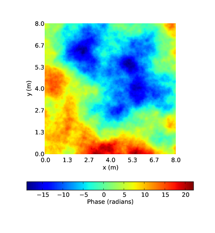
Figure 2.1: An example of the wavefront phase aberrations due to Kolmogorov turbulence. The wavefront (which is initially flat) is multiplied by this phase aberration map resulting in an aberrated wavefront. The spatial structure of the phase is fractal and so it looks the same on all scales. The magnitude of the phase aberrations depends on the strength of the turbulence.
2.1.2 Non Kolmogorov atmospheric turbulence
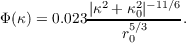
There is some evidence to suggest that the atmosphere does not always obey Kolmogorov’s 11/3 power law (e.g. [19, 20, 21]). It is sometimes found to be lower than 11/3 but rarely higher. Boreman and Dainty [22] generalised the 3D power spectrum for any power exponent, β. The generalised phase power spectrum takes the form, [22]
 | (2.11) |
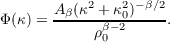
where Ωn2 is the refractive index structure constant with units of m3-β, Bβ is a coefficient which keeps consistency between the power spectrum and structure function. Φ(κ) can also be stated as,
 | (2.12) |
where ρ0 is the generalised coherence length and is analogous to the Fried parameter, r0, and Aβ is a coefficient chosen such that the piston subtracted wavefront variance over a pupil diameter D = ρ0 is equal to 1 radian2. The structure function is then [18],
 | (2.13) |
where γβ is another constant that keeps consistency between the power spectrum and structure fucntion and is given by,
![β-1[ (β+2)]2 (β+4)
2----Γ---2----Γ---2---
γβ = (β) .
Γ 2 Γ (β +1)](/wp-content/uploads/sites/167/2021/04/thesis18x.png) | (2.14) |
If β=11/3, i.e. the Kolmogorov case, this will reduce down to the constant in Fried’s structure function of 6.88 (equation 2.9).
Figure 2.2 shows an example of the phase aberration from a generalised spectrum with β = 9/3. The figure can be compared to the Kolmogorov example in figure 2.1. A lower β indicates more power on smaller spatial scales.
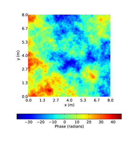
Figure 2.2: An example of the wavefront phase aberrations for non–Kolmogorov turbulence. In this case β = 9∕3.
2.1.3 Inner and Outer Scale
Although the previous equations are not valid at the limits of scales, i.e. very large and very small scales, this can often be ignored as a telescope acts as a spatial filter so that large scale fluctuations have little effect and small scale fluctuations contain very little energy. However, measured values of the outer scale vary between 1 m and 100 m [23]. At the lower end of this range there is an overlap with the size of modern astronomical telescopes and so should be included in AO modelling. The von Karman spectrum is a modified version of the Kolmogorov spectrum to take into account the finite outer scale, [18]
 | (2.15) |
where κ0 = 2π∕L0, or in terms of r0,
 | (2.16) |
The generalised spectrum becomes,
 | (2.17) |
or
 | (2.18) |
Due to the power law in Kolmogorov’s model there is very little power at small length scales and so the inner scale can usually be safely ignored. However, for completeness, the inner scale of optical turbulence has been measured to have values between 1 and 10 mm [24, 14] and the Von Karman equation including the inner scale is, [25]
 | (2.19) |
where κm2 = 5.92∕l0. Figure 2.3 shows the power spectrum of Kolmogorov, non–Kolmogorov and Von Karman turbulence with inner and outer scales of 5 mm and 20 m respectively.
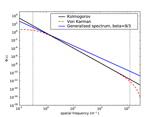
Figure 2.3: Example power spectra for Kolmogorov and non–Kolmogorov turbulence. The black line shows the standard Kolmogorov power spectrum with an exponent, β = 11∕3. The blue line is the generalised spectrum with β = 9∕3. This turbulence will have more energy on smaller scales and less energy on larger scales. The red dashed line is the Von Karman spectrum, which includes the inner and outer scale of turbulence. At spatial scales larger than the outer scale the power converges and drops to zero at scales smaller than the inner scale due to the dissipation of turbulent energy. The dotted lines indicate the spatial wavenumbers corresponding to inner and outer scales. The scale of the power spectrum is arbitrary and depends on the strength of the turbulence.
2.2 Imaging through turbulence
In the absence of turbulence the wavefront at the entrance pupil of a telescope will be flat. A flat wavefront would propagate through the telescope optics and focus to a diffraction limited point spread function (PSF). The full width at half maximum (FWHM) of the diffraction limited PSF will be [26],
 | (2.20) |
where D is the diameter of the telescope. The imaging resolution according to the Rayleigh criterion is,
 | (2.21) |
and is inversely proportional to the telescope diameter.
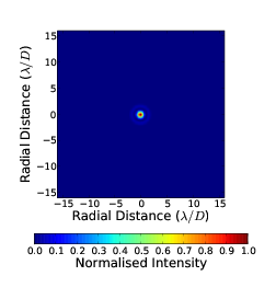
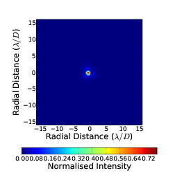
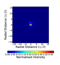
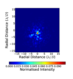
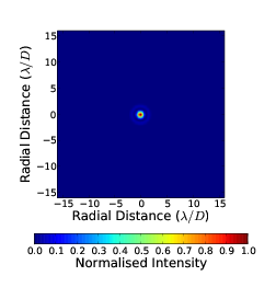
An image is formed by the interference of the light from every part of the wavefront with every other part. The refractive index fluctuations in the turbulent atmosphere induces an optical path difference between different parts of the wavefront. The focussed image will therefore not simply be a diffraction limited spot but constructive interference around the central region will also occur. The turbulence perturbed wavefront will cause the short exposure image to break up into a number of speckles. Each one approximately the same size as the diffraction limited PSF. However, the area over which the speckles are spread will depend on the integrated strength of the optical turbulence along the propagation path of the wavefront, quantified by the Fried parameter, r0. For example in an atmosphere/telescope system with the ratio of D∕r0 = 10 the speckles will be spread over an area approximately 10 times larger than the diffraction limited PSF. Figure 2.4 shows example images for a diffraction limited system and turbulence limited systems with D∕r0 = 1, 4 and 10.
 |  |
| (a) | (b) |
 |  |
| (c) | (d) |
Figure 2.4: Example simulated images through a diffraction limited system (a) and a turbulence limited system with D∕r0 = 1 (b), 4 (c) and 10 (d). It is seen that the image breaks up into a number of speckles. Each of these speckles is approximately the size of the diffraction limited PSF but they are spread over an area D∕r0 times larger. The intensity is normalised to the peak intensity of the diffraction limited case.
The phase variance across the aperture can be calculated using [17],
 | (2.22) |
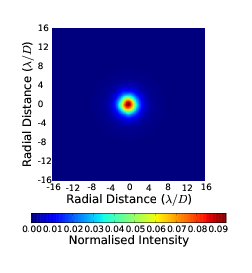
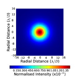
If a telescope has a diameter less than r0 then the phase variance will be very small and will be effectively diffraction limited even with the presence of optical turbulence. If the telescope diameter is larger than r0 then there will be significant phase aberrations in the wavefront which will cause the image to appear speckled. These speckles will process and evolve with time as the phase aberrations change due to the atmosphere crossing the field of view of the telescope. In a long exposure the speckles will add together to produce a large (in angular extent) low level halo. Figure 2.5 shows example long exposure PSFs for diffraction limited and D∕r0= 1, 4 and 10 systems.
 |  |
| (a) | (b) |
 |  |
| (c) | (d) |
Figure 2.5: Example simulated long exposure images through a diffraction limited system (a) and a turbulence limited system with D∕r0 = 1 (b), 4 (c) and 10 (d). The PSF is spread oven an area approximately D∕r0 times larger. The intensity is normalised to the peak intensity of the diffraction limited case. The images shown are the sum of 100000 unique images from random phase screens.
The FWHM of the turbulence degraded image is,
 | (2.23) |
this value is independent of the telescope diameter and is known as the atmospheric seeing angle. The angular resolution will also be limited by the atmosphere,
 | (2.24) |
In contrast to the short exposure PSF which is a direct result of the exact form of the wavefront perturbations the long exposure is formed by averaging over many instances of the turbulence and it is therefore possible to analytically calculate the shape of this statistical PSF from the atmospheric parameters. The long exposure PSF assuming on-axis observations can be calculated by,
![P SF = F [M T Fatmos × M TF tel],](/wp-content/uploads/sites/167/2021/04/thesis39x.png) | (2.25) |
where MTFatmos is the atmospheric modulation transfer function and MTFtel is the telescope modulation transfer function.
In the case of diffraction limited imaging the first term can be ignored and the PSF is only dependant on the telescope modulation transfer function which is given by the autocorrelation function of the pupil function. In strong seeing conditions the cut off frequency of the telescope MTF is much higher than the atmospheric MTF and the second term can therefore be ignored (figure 2.6).
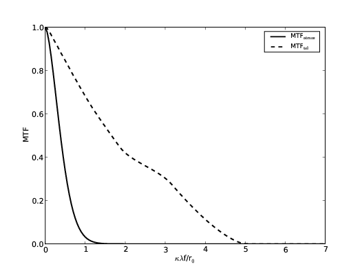
Figure 2.6: Modulation transfer functions for the telescope, MTFtel, dashed line and the atmosphere, MTFtel, solid line. The cut off frequency of the telescope MTF is much higher than that of the atmospheric MTF. For this reason the telescope MTF can be ignored in equation 2.25. In this case r0 = 0.2 m and D = 1.0 m.
The atmosphere acts as a spatial filter. In the absence of this filter and a perfect imaging system all of the information from the object would be replicated in the image. However, the atmosphere reduces the resolution, it removes information about the object. The atmospheric transfer function, MTFatmos(r), tells us how spatial frequencies in the object convert to spatial frequencies in the image and is given by the auto-covariance function of the wavefront,
 | (2.26) |
or, using equation 2.2,
![M T Fatmos(r) = ⟨exp(i[ϕ(ε)- ϕ(ε+ r)])⟩.](/wp-content/uploads/sites/167/2021/04/thesis42x.png) | (2.27) |
Roddier (1981) [14] shows that this can be re-written as,
 | (2.28) |
Using equation 2.7 MTFatmos(r) can now be written as [27],
 | (2.29) |
where the MTF is shown as a function of separation in the pupil, r, and Dϕ(r) is the phase structure function. We can now relate the phase structure function to measurable atmospheric parameters using Kolmogorov’s turbulence models (using equation 2.9). The seeing limited point spread function PSF is then approximated by,
![[ ( ( ) )]
PSF = F exp - 3.44 r-5∕3 , r ≪ L0.
r0](/wp-content/uploads/sites/167/2021/04/thesis45x.png) | (2.30) |
In the intermediate case, when 1 ≤ D∕r0 ≤ 4 the telescope modulation transfer function must also be included,
![[ ( ) ]
( r-)5∕3
P SF = F exp - 3.44 r0 M TF tel , r ≪ L0.](/wp-content/uploads/sites/167/2021/04/thesis46x.png) | (2.31) |
As r approaches L0 the power in the low order modes will be reduced leading to an increase in image quality. This can be included in the analytical model by using a von Karman power spectrum rather than the Kolmogorov model.
2.3 Adaptive Optics
The turbulent atmosphere causes phase variations across a wavefront propagating from an astronomical object to a ground based telescope. It is well known that these distortions degrade the imaging performance of the telescope (see section 2.2) and the whole field of adaptive optics (AO) has been developed to ameliorate these distortions.
Figure 2.7 shows a simple diagram of an AO system. The distorted wavefront is corrected by a deformable mirror. The wavefront sensor is usually placed after the deformable mirror in the optical train so that it measures only the residual wavefront error which is then added to the previous correction in order to converge to a better correction.
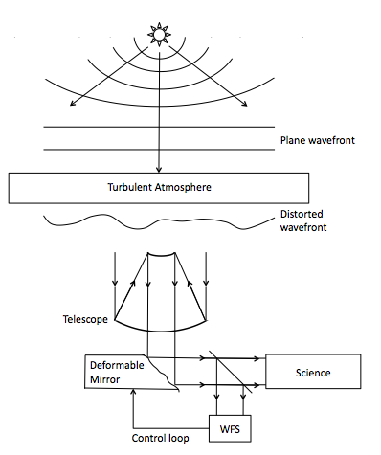
Figure 2.7: The light emitted from a star is initially spherical. After propagating the vast distance to the top of the Earth’s atmosphere the wavefront is essentially flat. It is only in the last few 10’s of kilometres that the wavefront gets distorted by the refractive index perturbations in the atmosphere. Adaptive optics uses a deformable mirror to flatten the wavefront, potentially restoring the diffraction limited potential of the telescope. Most AO systems are closed loop, the wavefront sensor is positioned after the deformable mirror and measures the residual wavefront error which is passed back to the deformable mirror.
However, no AO system is perfect and the partially corrected point spread function (PSF) from a typical AO system consists of a diffraction limited core sitting on top of a much broader halo. The short exposure halo is made up from speckles which are averaged in a long exposure to produce a large (in angular extent) low level plateau which can limit the achievable signal to noise ratio of the detection of faint objects around bright stars.
2.3.1 Wavefront sensing
Wavefront sensors are used to measure the phase across a wavefront. There are many varieties of wavefront sensors, each with their own strengths and weaknesses. The adaptive pupil mask and SLODAR which are described in later chapters both use Shack–Hartmann wavefront sensors. Therefore only the Shack–Hartmann is described here.
The Shack–Hartmann wavefront sensor uses an array of lenslets (or subapertures) positioned in the pupil plane of the telescope. A flat wavefront will illuminate these lenslets and create a uniform pattern of spots at the focus. If a lenslet is illuminated with a wavefront containing a local tilt in the angle of arrival the spot will deviate from its central position. The amplitude of this deviation is a measure of the local tilt on each subaperture. The centroid positions of all the spots can then be used to reconstruct the phase map in the wavefront. Figure 2.8 is a simple diagram of a Shack–Hartmann wavefront sensor.
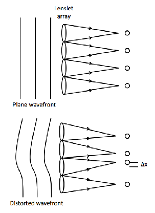
Figure 2.8: A flat wavefront illuminating the lenslet array will create a regular array of spots as shown in the top diagram. A distorted wavefront will illuminate different subapertures with a different angle of arrival resulting in a distorted spot pattern. The excursion of the spot from its central position, Δx, is a measure of the mean tilt across the subaperture.
2.3.2 Imaging with Adaptive optics
For partially corrected wavefronts the structure function is no longer given by equations 2.9 and 2.10. An AO system will reduce the phase structure function for low spatial frequencies as the deformable mirror can be manipulated in such a way as to correct for them. Greenwood [28] proposed a model which can be used to analyse the effect of an AO system on an aberrated wavefront. The model predicts the effect of a segmented AO system on the wavefront without inferring any aperture. This model is an approximation to a real AO system with an infinite aperture which has no edge effects and no noise. The model uses a high pass filter, H(κd∕2), to remove these low spatial frequencies as shown in figure 2.9 (a),
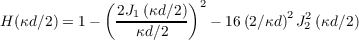 | (2.32) |
where d is the diameter of the subapertures and Jn is a Bessel function of the first kind of order n. The partially corrected phase structure function is given by Greenwood [28] as,
![∫ ∞ Dϕ,AO(r) = 4π [1- J0(κr)]Φ(κ)H (κd∕2)κdκ. 0](/wp-content/uploads/sites/167/2021/04/thesis50x.png) | (2.33) |
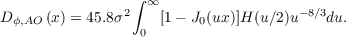
Equation 2.33 can be re-arranged to,
![∫ 5∕3 ∞ -8∕3 D ϕ,AO (x) = 6.14(d∕r0) 0 [1- J0(ux )]H (u∕2)u du](/wp-content/uploads/sites/167/2021/04/thesis51x.png) | (2.34) |
where x = r∕d and u = κd in order to bring the d∕r0 term to the front and so that the integral does not depend on the atmospheric parameters. The phase variance of a tip/tilt corrected wavefront is σ2 = 0.134(d∕r0)5∕3 and so it can be seen that the coefficient of the structure function is determined by the wavefront variance and equation 2.34 can be written as,
Due to the spatial filter term the structure function will saturate at some spatial frequency. The frequency at which this occurs is determined by the parameters of the AO system and the amplitude of the saturation is set by the coefficient and is therefore dependant on the wavefront phase variance. Increasing r0 will reduce the wavefront variance and lower the saturation level of the structure function. Figure 2.9(b) shows the partially corrected structure function for d∕r0 = 1 and it is seen that this converges to a value of 0.268 which is consistent with 2σ2. From this we can confirm that equation 2.34 converges to 2σ2 and for a partially corrected wavefront equation 2.10 becomes
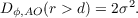
 |  |
| (a) | (b) |
Figure 2.9: Theoretical plots to show the effect of an AO system on the wavefront structure function. (a) is the AO high pass filter function as defined by Greenwood [28]. Low spatial frequencies are removed by the AO system and high spatial frequencies propagate. (b) shows the theoretical uncorrected structure function (green line) and the theoretical partially corrected structure function (blue line). The simulated structure functions are shown in black and red. The simulated partially corrected structure function is larger than the theoretical value as the simulation includes realistic noise sources which are not in Greenwood’s theoretical model. The simulated uncorrected structure function underestimates the phase variance at large separations as low order modes are not properly averaged. The partially corrected structure function saturates when r > d (d = 0.5 m in this case) as large spatial scale deformations (low spatial frequencies) have been removed by the AO system as seen in (a).
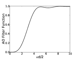
The AO MTF can then be found by placing equation 2.35 in equation 2.29. Figure 2.10 (a) shows the MTFatmos for a number of values of d∕r0 after AO correction. The curves can be decomposed into a Gaussian with a dc bias. The atmospheric component of the PSF will be a central peak defined by the dc offset plus a Gaussian halo with width inversely proportional to the width of the MTFatmos Gaussian component. As all the curves correspond to the same total intensity the fraction of energy within the core is given by the value of the dc offset, in this case the convergent value of MTFatmos, and when the phase variance is low (< 1.6 radians2) the Maréchal approximation tells us that this constant is equal to the Strehl ratio, which is defined as the ratio of the peak intensity of the of the aberrated image to that of the diffraction limited PSF.
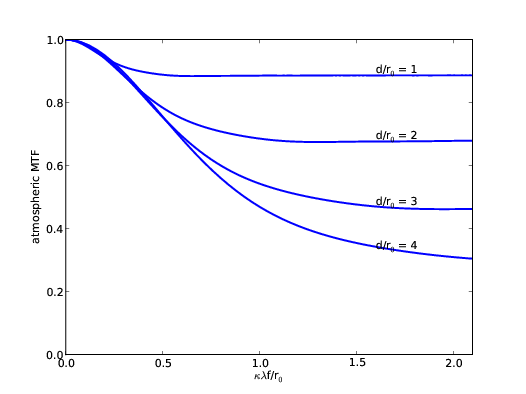
Figure 2.10: The atmospheric modulation transfer function after AO correction depends on the wavefront variance, defined by the d/r0 ratio. The plot shows the atmospheric modulation transfer function for a range of d/r0 values. A lower ratio means the AO system is capable of better correction and so will converge at a higher level. Equation 2.29 states that the MTFatmos converges to exp which using the Maréchal approximation indicates the fraction of energy within the diffraction limited core.
As the residual wavefront variance after AO correction can be small the telescope MTF must now be included. The analytical PSF is,
![[ ( ∫ ∞ ) ]
PSF = F exp - 3.07(d∕r)5∕3 [1- J (ux)]H (u∕2)u -8∕3du M TF .
0 0 0 tel](/wp-content/uploads/sites/167/2021/04/thesis58x.png) | (2.37) |
2.3.3 AO Taxonomy
All the information above refers to single conjugate AO (SCAO). This is a specific type of AO system where the deformable mirror is conjugate to the telescope pupil and has only a very small corrected field of view. Away from the guide stars (which are used for the wavefront sensing) the correction quickly deteriorates due to the small isoplanatic angle associated with the atmospheric turbulence. Extreme AO systems for high contrast imaging of extrasolar planets for example use SCAO as they are only attempting to correct a very small field of view. Other AO schemes have been developed to increase the homogeneously corrected field of view although these often result in a worse correction. Ground layer AO (GLAO) [29] can be used to improve image resolution over a wide field of view by correcting only for turbulence close to the ground. Any turbulence at higher altitudes will limit the magnitude of the correction. Measurements have shown that in many astronomical sites the ground layer can contribute up to 50% of the turbulence strength [13]. By removing this component a large improvement in image quality can be obtained. To increase the imaging resolution more complex systems, such as Multi-Conjugate AO (MCAO) [30], correct for multiple layers including the ground layer. In this way the AO system can deliver a large highly corrected field. Other variants exist but only those mentioned are discussed in this thesis.
2.4 Photometry through atmospheric turbulence
High precision fast photometry is key to several branches of research including (but not limited to) the study of extrasolar planet transits (e.g. [31]), stellar seismology [32] and the detection of small Kuiper belt objects (e.g. [33]). The difficulty with such observations is that, although the targets are often bright, the amplitude of variability is often very small (typically millimagnitudes or less) and hence the noise is not limited by the detector or sky but by intensity fluctuations (scintillation) produced by the Earth’s atmosphere. For this reason fast photometers are generally put in space (e.g. CoRoT, Kepler and PLATO).
Extrasolar planetary transits can be detected from the ground. However the measurement of the secondary eclipse (i.e. where the planet goes behind the star) is a challenge. Such observations are crucial, as only the secondary eclipse can give information on the planetary atmosphere, including the temperature and albedo [34]. Secondary eclipses were detected for the first time from space in 2005 using Spitzer at 3 μm [35]. There has been a great deal of effort to detect secondary eclipses from the ground, but for years no detections were made (in large part due to scintillation noise). Finally, in 2009, the first ground-based detections were made, but these relied on near-IR measurements and had to target the most bloated, closest (to their host star) exoplanets to maximise the eclipse signal [36]. Since then a few other exoplanets have had secondary eclipses detected from the ground in this way. As noted by Deming & Seager [6], secondary eclipses recorded in visible light in addition to IR measurements are crucial if we are to understand the relative contribution of thermal emission and reflected light, and the planetary albedo.
Time averaging the intensity will reduce the scintillation noise by an amount proportional to the square root of the exposure time [37]), but this will often result in saturating the CCD which then requires de-focusing the telescope to distribute the image of the star over more pixels. De-focusing has certain advantages, such as reducing the impact of pixel-to-pixel and intra-pixel sensitivity variations, but it also significantly increases the sky and CCD readout noise [38]. In addition, de-focussing is not routinely possible on some telescopes (e.g the VLT) and it can not be done with crowded fields. More importantly for fast photometry, time averaging can also only be used in circumstances where the intrinsic variability of the target has a much longer time scale than the scintillation. As scintillation is caused by the spatial intensity fluctuations crossing the pupil boundary, the time scale is determined by the wind speed of the turbulent layer. Dravins et al. [39, 40, 37] studied the temporal autocorrelation of the scintillation pattern at astronomical sites and found that the power is mainly located between 10 and 100 Hz but actually spans many orders of magnitude.
Differential photometric measurements can be made by normalising with a nearby comparison star (e.g. [41]). This is not to reduce the scintillation but to correct for transparency variations in the atmosphere. However, this actually makes the scintillation noise worse as it is inherently caused by high altitude layers and therefore will have a very small angle of coherence (defined here as the isophotometric angle, analogous to the isoplanatic angle for wavefront phase) in the optical (typically ~ 1′′).
2.4.1 Scintillation
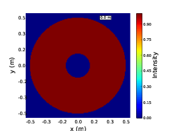
The observational effects of Scintillation have been well documented [42]. High altitude turbulence in the atmosphere distorts the plane wavefronts of light from a star, which is effectively at infinity. As the wavefronts propagate, these phase aberrations evolve into intensity variations. As the turbulent layer is blown across the field of view these “flying shadows” or intensity fluctuations move across the ground which we view with the naked eye as twinkling. Wavefronts incident on a telescope pupil have both phase variations, caused by the integrated effect of light passing though the whole vertical depth of the atmosphere, and intensity variations, caused predominantly by the light diffracting through high altitude turbulence and interfering at the ground. Example simulated spatial intensity fluctuations are shown in figure 2.11.
Figure 2.11: An example of a simulated pupil image with scintillation fluctuations. In this case the turbulet layer was at an altitude of 10 km and the telescope diameter was 1 m.
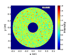
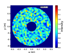
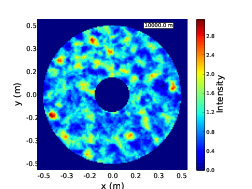
As a wavefront propagates away from a turbulent layer the spatial intensity fluctuations become larger both in terms of intensity and spatial extent. The characteristic spatial scale of the fluctuations is given by the radius of the first Fresnel zone, rF =  . This is not dependant on the strength of the layer which only effects the magnitude of the intensity fluctuations and not their spatial scale. Figure 2.12 shows example simulated pupil images for a several propagation distances
 |  |
| (a) | (b) |
 |  |
| (c) | (d) |
Figure 2.12: Example pupil images for no turbulence (a) and a turbulent layer at 1 km (b), 5 km (c) and 10 km (d). As the wavefront propagates further away from a turbulent layer the intensity fluctuations grow larger both in terms of spatial scale and intensity.
and figure 2.13 shows the mean spatial covariance functions. The covariance functions have a minimum at the Fresnel radius for each propagation distance.
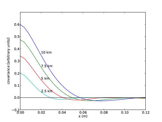
Figure 2.13: Spatial covariance plots for scintillation pupil patterns. By allowing the wavefront to propagate further the spatial intensity fluctuations become larger (figure 2.12). The characterisitc spatial scale of these fluctuatios is given by the Fresnel radius, rF =  . The spatial covariance has a minimum corresponding to this distance.
The scintillation does modify the phase power spectrum. It is modulated by a cosine squared with a frequency set by the altitude of the turbulent layer,
 | (2.38) |
Figure 2.14 shows the modified phase power spectrum.
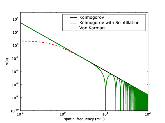
Figure 2.14: Scintillation modified phase power spectrum. In this case a turbulent layer was assumed to be at 10 km and the wavelength is 500 nm.
As the modifications are restricted to high spatial frequencies which contain little power the net effect on an optical image is small. Phase variations are normally more significant as they dramatically affect the imaging performance of the telescope, and this has lead to the development of adaptive optics (see section 2.3). The intensity variations across the pupil are effectively averaged together when the light is focussed and therefore have less effect. A larger aperture implies more spatial averaging (which is why stars twinkle less when observed through a telescope than with the naked eye). However, these small intensity fluctuations do become significant when one is concerned with high precision photometry.
Consider now the effect of these intensity variations in more detail. If we ignore diffraction, then a flat wavefront which is the same size as the telescope pupil at a given high altitude, in the absence of atmospheric turbulence, will propagate in a direction normal to the wavefront and will all be collected by the telescope pupil. Now consider the effect of atmospheric distortion. Phase aberrations cause different rays across the wavefront to propagate in different directions, which interfere to produce scintillation. This in itself is not a significant problem for photometry, as the integrated intensity across the pupil is the same. The problem occurs either when high altitude areas of the wavefront, which in the absence of turbulence would fall outside of the telescope pupil, can be diffracted by the turbulence and interfere to cause intense regions within the pupil area, or conversely when high altitude areas of the wavefront which are diffracted by the turbulence interfere to cause intense areas at the ground outside of the telescope pupil are lost. These effects lead to an increase and decrease in intensity, respectively, and at any one instant both of these effects will be occurring, producing an overall change in intensity.
Scintillation is generally quantified by the intensity variance, named scintillation index, and can be calculated by summing the difference of the intensity, I(t,λ), from the expected value, ⟨I⟩,
 | (2.39) |
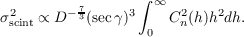
The scintillation index, σscint2, is dependent on the height of the turbulent layers, h, the refractive index structure coefficient, Cn2(h), the wavelength, λ, and the zenith distance and can be predicted using the theoretical model described by Dravins et al. , [40],
 | (2.40) |
This expression assumes that there is no temporal or spatial averaging and so is only valid for telescopes with a pupil diameter less than the characteristic spatial correlation scale of the amplitude fluctuations, i.e. D < rF (see figure 2.13).
Larger telescopes average out the small scale spatial fluctuations. If the pupil is much larger than the Fresnel radius (D ≫ rF) equation 2.40 is modified to
 | (2.41) |
The scintillation index is then independent of wavelength and proportional to the strength of the turbulent layer and the altitude of the turbulent layer squared.
The scintillation index given in equation 2.41 is only valid for very short exposures where there is no temporal averaging, i.e. the exposure time has to be less than the crossing time of the intensity fluctuations. The crossing time, tc can be calculated as tc = D∕vw, where vw is the velocity of the turbulent layer. If the exposure time, t, is greater than the crossing time the scintillation index is modified to [43],
 | (2.42) |
where V (h) is the velocity of the turbulent layer at altitude h.
2.5 Numerical Simulations
2.5.1 AO simulations
The existing Durham AO simulation platform [44] has been developed to test novel real time correction ideas. The atmosphere is modelled by a number of phase screens located at discrete altitudes. In reality the structure of the turbulent layer will change with time as it mixes and evolves. This will be on time scales longer than the crossing time of the turbulent layer and so we assume that the atmosphere ‘screen’ is frozen as it moves across the pupil (Taylor’s approximation).
The phase screens (ϕh) are derived using equations based on those discussed by Ellerbroek [45] and are generated by filtering white Gaussian noise to obtain a random field with the correct second order statistics. This is achieved by multiplying a randomly generated repeatable white noise field (r(κ) + ir′(κ), where κ is the spatial frequency variable and r and r′ are zero mean, unit variance random fields) by a spatial power spectrum, Φ(κ), of the turbulence required. The spatial power spectrum is calculated as follows,
 | (2.43) |
where W is the width of the phase screen and L0 is the outer scale of the turbulence. The equation shown will calculate the spatial power spectrum of von Karman turbulence. Kolmogorov statistics are achieved by setting the turbulence outer scale, L0, to infinity, removing the second term in the spatial power spectrum. The resulting product is 2D Fourier transformed (denoted by  ) and the real part is multiplied by a constant therefore,
![( ) 5
PS = 0.1√517- W-- 6 ℜF [∘ Φ(κ)(r(κ)+ ir′(κ))].
2 r0](/wp-content/uploads/sites/167/2021/04/thesis74x.png) | (2.44) |
The constant is used to scale the strength of the phase screen, so that different layers within the atmosphere can be parameterized with a unique Fried parameter, r0. The phase screen is expressed in terms of a phase shift corresponding to the wavelength of the wavefront passing through it rather than an optical path difference.
A unique phase screen is generated for each turbulent layer. If only one on-axis target is required the phase aberrations of each layer are summed assuming geometrical optics. The simulation is capable of multi object handling in which case the phase aberrations are summed through different areas of each phase screen depending on its altitude. The phase screens are ‘infinite’ in extent in that new areas are calculated during runtime instead of simply wrapping large phase screens.
The simulation is modular and passes only phase information between the modules. This simplifies the process of developing the simulation to include new test modules. For the work presented in this thesis the simulation was modified to pass complex amplitudes between modules and a four-quadrant phase mask coronagraph module was developed to test ideas for high contrast imaging.
2.5.2 Fresnel Simulations
The Fresnel propagation simulation has been developed from a version by Tim Butterley and Richard Wilson. The Fresnel diffraction integral is given by [46],
![i ∫
Ψ(x′,y′,0) = --exp(ikz) Ψ (x,y,z)
λz ( [ ])
exp ik- (x- x′)2 + (y - y′)2 dx ′dy′
2z](/wp-content/uploads/sites/167/2021/04/thesis75x.png) | (2.45) |
where Ψ

and Ψ

are the wave functions in the diffraction plane at co-ordinates x,y,z and observation plane at co-ordinates x′,y′,0 respectively and z is the propagation distance. This can also be expressed as a convolution of the wave function with a Fresnel diffraction kernel as,
 | (2.46) |
where ⊗ denotes a convolution and K(z) is the Fresnel propagation kernel and is given by,
![( [ ])
K (z) = -iexp (ikz)exp ik (x - x′)2 + (y- y′)2 .
λz 2z](/wp-content/uploads/sites/167/2021/04/thesis79x.png) | (2.47) |
In the simulation the convolution can be performed with fourier transforms,
 | (2.48) |
In the case of atmospheric propagation between a number of turbulent layers, at each layer the wave amplitude will be multiplied by the complex amplitude of the turbulent layer,
 | (2.49) |
where ϕh is the phase screen located at altitude h. The modified wave amplitude is then propagated to the next layer via a convolution with the Fresnel kernel. The intensity distribution at plane z, I , is equal to the wave amplitudes squared.
Periodic phase screens are used in this simulation rather than the ‘infinite’ phase screens discussed in section 2.5.1. This is because the fourier transforms require periodicity to avoid discontinuities in the resulting wavefront. The phase screens can then be ‘wrapped’ and translated across the telescope field of view.
2.6 Site Characterisation
Knowledge of the vertical profile of optical turbulence at observatory sites is of growing importance for the application of increasingly sophisticated adaptive optical (AO) correction systems for astronomy. The latest AO systems address correction of individual turbulent layers in the atmosphere, in order to overcome the effects of anisoplanatism and thereby increase the corrected field of view. For example Ground Layer AO (GLAO) [29] can be used to improve image resolution over a wide field of view by correcting only for turbulence close to the ground. In this case the size of the homogeneously corrected field of view is determined by the thickness and vertical distribution of the ground-layer turbulence. To increase the imaging resolution, more complex systems, such as Multi-Conjugate AO [30] correct for multiple layers including the ground layer. Hence detailed knowledge of the optical turbulence profile, and of the ground layer in particular, is critical in order to predict, model and optimise the performance of the latest and next generation of AO instrumentation.
In addition to the optimisation of AO systems, turbulence profiling is required for site testing and selection for the next generation of large telescopes [47]. It may be possible to shield the telescope from the majority of the turbulence with novel dome design or even by building the telescope above the surface layer of turbulence. Various observations have shown that the surface layer is typically strong [12, 13], contributing a significant fraction of the total seeing aberration, but also thin, as observed at Dome C in Antarctica [48]. Previous measurements of the optical turbulence profile by SLODAR (SLope Detection And Ranging) [9] at the Cerro Paranal observatory have also shown that the surface layer (approx. the first 100m in altitude) contains a large fraction of the total turbulence [7]. However, SLODAR was unable to resolve the surface layer so that its true thickness could not be determined.
The surface layer is the lowest turbulent layer in the atmosphere. It is primarily caused by the temperature differences between the ground and the air. However, wind flow around obstacles such as artificial structures, large rocks and mountains also result in turbulent flow leeward of the obstacle. The surface layer is therefore highly dependant on local topography and is defined as the maximum altitude that these surface effects have influence and is generally considered to be less than ~100 m. The surface layer completely dominates day time solar observations and at Dome C, Antarctica [48].
The ground layer is a term prevalent with adaptive optics scientists particularly those interested in GLAO. The thickness of the ground layer is defined so that it is completely compensated by a GLAO system and is often quoted in the literature as extending up to approximately 1 km. The thinner this layer is the greater the isoplanatic angle of the AO system. The high altitude turbulence in the “free atmosphere” is uncorrected and degrades the resolution. Turbulence at altitudes between the ground layer and the higher free atmosphere is partially corrected by a GLAO system and is termed the “gray zone”.
A number of techniques for profiling of ground-layer turbulence have been demonstrated in recent years. These include optical methods based on measurement of the fluctuations of intensity (scintillation) induced by the turbulent layers, including LOLAS (LOw LAyer SCIDAR) [49], HVR-Generalized SCIDAR [12] and the lunar scintillometer (LuSci) [50]. “Generalised” SLODAR has been demonstrated to increase the resolution of a SLODAR system. By re-conjugating the lenslet array between observations it is possible to increase the resolution of the system [51]. However, this technique assumes the turbulence is constant during re-conjugation. SODAR (SOnic Detection And Ranging) acoustic profilers have also been used for ground-layer studies in astronomical site testing [52].
2.7 Turbulence Monitoring Instrumentation
A number of instruments are mentioned in this thesis and an outline of some of them is presented below.
2.7.1 Differential Image Motion Monitor (DIMM)
The DIMM is used to obtain an unbiased measurement of the seeing. The DIMM is a well tested and trusted instrument. It measures the image motion of two copies of a star through two small apertures (~10 cm) separated in the pupil. The differential image motion is converted into a seeing angle. The differential method means that it is insensitive to tracking errors. The DIMM was developed by ESO for the site selection campaign for the VLT by Sarazin and Roddier [26] and is now used at most major observatories around the world. The DIMM does not provide a turbulence profile.
2.7.2 Multi-Aperture Scintillation Sensor (MASS)
The MASS uses the correlation between the stellar scintillation patterns at varying scales to estimate the turbulent profile. As it works with scintillation which is predominantly caused by high altitude turbulence the MASS is not sensitive to surface layer turbulence. The ESO MASS piggy backs on the DIMM telescope and provides turbulence strength estimates for 6 bins centred at h = 0.5, 1, 2, 4, 8 and 16 km with a resolution of h∕2 [53]. By summing the total MASS turbulence strength and subtracting from the DIMM measurement it is possible to calculate the ground layer turbulence strength.
2.7.3 Lunar Scintillometer (LuSci)
LuSci is similar to MASS in that it measures the correlation of scintillation on varying scales to estimate the turbulence strength at different altitudes. However, LuSci uses photodetectors to measure the intensity rather than annular apertures and uses the Moon as its target to measure the profile of the surface turbulent layer. It is well known that scintillation from extended source is dominated by the surface layers [54]. The effects of a turbulent layer at a high altitude is averaged as the light cone is large. For example the Moon will illuminate an area of turbulence nearly 100 m across at an altitude of 10 km above the ground. The light cone through the lower layers is small (approximately 0.1 m at 10 m) and so will actually result in more scintillation. Beckers was the first to use this phenomenon to measure the surface layer turbulence for day time solar astronomy using the sun as its target with SHABAR [55]. Using the moon creates additional challenges, not only is it only useable four days either side of full moon but the response of the instrument also changes with its phase.
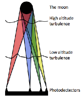
Figure 2.15: Diagram of the LuSci geometry. The photodetectors are positioned such that correlation between different detectors corresponds to turbulence of a certain altitude. As the moon is an extended object the instrument is most sensitive to low altitude turbulence.
2.7.4 SCIntillation Detection And Ranging (SCIDAR)
SCIDAR is an optical triangulation technique. A turbulent layer at some altitude, h, illuminated by two stars with angular separation, θ, will result in two copies of the same wavefront aberration on the ground separated by a distance hθ. There will therefore be a peak in the time averaged spatial covariance function at a separation corresponding to this distance. The amplitude of the correlation peak will correspond to the strength of the turbulence. The velocity of the layer can be found by calculating the cross covariance maps with a temporal offset. The turbulent layer will traverse across the field of view of the telescope as it is blown by the wind. This means that the wavefront aberration will also appear to flow across the pupil. By calculating the time averaged covariance of the aberrations of one star, at time t, with the aberrations from the other star a short time later, t + δt, the covariance peak will move. The distance the peak moves in δt can be converted to a wind speed.
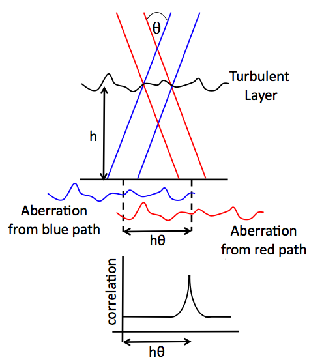
Figure 2.16: If a turbulent layer at height, h, is illuminated by two stars of angular separation, θ, then two copies of the aberration will be made on the ground separated by a distance hθ. By cross correlating either the centroid positions from a Shack–Hartmann wavefront sensor (SLODAR) or the intensity patterns (SCIDAR) we can triangulate the height of the turbulent layer and the amplitude of the correlation peak corresponds to the strength of the layer.
SCIDAR uses the spatial intensity fluctuations caused by the turbulent layer as the aberration pattern. As scintillation is dominated by high altitude turbulence conventional SCIDAR is incapable of measuring the turbulence strength close to the ground. A modification of SCIDAR called generalised SCIDAR [10] has been developed to avoid this limitation. Generalised SCIDAR conjugates the analysis plane below the ground level. This allows the wavefront to propagate through the optical system and develop measurable scintillation.
The vertical resolution of SCIDAR is limited by the minimum separation of the autocorrelation peaks which can be determined. This in turn is set by the spatial scales of the turbulence. Therefore, in order to achieve high resolution profiling the telescopes need to be quite large (>1 m [49]). This limitation means that SCIDAR is not portable. Low Layer SCIDAR (LOLAS) [49] is a variant of SCIDAR and is implemented on a small portable telescope. It is used to profile the surface turbulent layer with high vertical resolution but a small number of resolution bins.
2.8 SLOpe Detection And Ranging (SLODAR)
SLODAR is a stereoscopic technique which has been developed to profile the vertical distribution of optical turbulence, Cn2(h). It is similar to SCIDAR except that instead of using the scintillation patterns the phase aberrations of the wavefront are used to profile the atmosphere. By triangulating the wavefront gradients for two target stars, measured using a Shack Hartmann wavefront sensor, we can estimate the altitude, strength and velocity of each turbulent layer up to a maximum altitude determined by the geometry of the system [9]. Figure 2.17 shows the geometry of the SLODAR method.
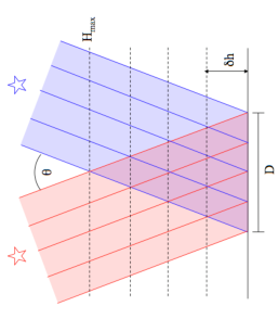
Figure 2.17: SLODAR geometry. θ is the angular separation of the target stars, D is the diameter of the telescope, Hmax is the maximum altitude that can be resolved and δh is the altitude resolution of the system.
The vertical resolution, δh, of the SLODAR system is given by,
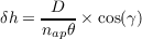 | (2.50) |
where D is the diameter of telescope aperture, nap is the number of subapertures subtended across the pupil, θ is the angular separation of the target stars and γ is the zenith angle of the observation. The air mass correction is required to convert between distance from the instrument to absolute altitude. The maximum altitude that can be resolved is then,
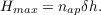 | (2.51) |
As the method is based on direct measurements of the wavefront phase gradient, it is relatively straightforward to calibrate in terms of the absolute optical turbulence profile. The technique can be applied to a small telescope as a portable turbulence profiler or to a large telescope to profile the turbulence with a very high vertical resolution.
2.8.1 SLODAR data analysis
A detailed description of the SLODAR data analysis method is given by Butterley et al. (2006) [56]. However, a review of the general technique is presented here for completeness. More details regarding the surface layer SLODAR (SL–SLODAR) system specifically is described in chapter 3.
The SLODAR data analysis pipeline begins by recording the wavefront sensor images for a few seconds with an exposure time of approximately 1–3 ms. These frames are stacked up until about 30 seconds of data has been collected which is then used to generate a single turbulence profile. The images are processed to remove the background and examined to locate any subapertures which are not illuminated in all of the data, this subaperture is then ignored from all further analysis. The Shack Hartmann wavefront sensor spots are found with Gaussian fitting to the average image and the centroid positions in each frame are calculated using standard centre of mass centroiding. The centroid streams may be temporally filtered at 1 Hz to remove the slowly evolving tube seeing [51]. The average centroid motion is removed from each frame of the data to avoid bias from telescope guiding errors and wind-shake.
The centroid slopes from the two stars are cross correlated and averaged to result in a 2D cross-covariance map. Figure 2.18 shows an example 2D auto-covariance and cross-covariance.
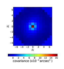 | 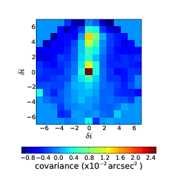 |
| (a) | (b) |
Figure 2.18: Example 2D auto-covariance (a) and cross-covariance (b) maps for SLODAR. This data was taken at Paranal on the night of 8th February 2009. The profile is recovered from a fit to the cross-covariance in the direction between the two stars, in this case in the upward direction. We can see strong correlation in the central bin indicating turbulence at the ground and another strong correlation at a separation, δi, of five subapertures indicating a turbulent layer at an altitude of 5 × D cos(γ)∕(nap × θ).
The cross covariance values on a line from the centre to the outer edge in the direction of the two stars tells us the centroid correlation as a function of displacement in the pupil in the direction joining the two target stars. In figure 2.18 the stars are aligned in the upward direction. Figure 2.19 shows a slice of the 2D cross-covariance in the direction of interest. The slice shows a strong peak at zero displacement signifying strong turbulence at the ground. There is also a second peak offset by approximately 5 subapertures, this shows that there is correlation in the centroid values at this separation and indicates a second turbulent layer at an altitude of 5 × D cos(γ)∕(nap × θ).
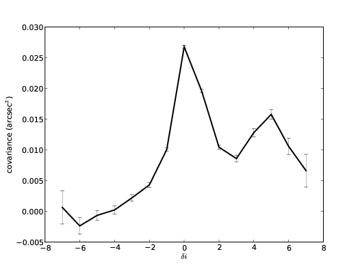
Figure 2.19: 1D slice of the cross-covariance function in the direction between the two stars. δi is the separation in the pupil in units of subapertures. The errors increase with greater separations as fewer subapertures overlap.
The cross-covariance function peaks at positions corresponding to the altitude of the turbulent layers but the shape of this function is not the turbulent profile. The profile is recovered by fitting the cross-covariance function with the response functions of the instrument. The auto-covariance function could be used as an estimate of the response of SLODAR to turbulence. However, the process of removing the average centroid motion also removes any common tilt motion induced by the atmosphere which means that a simple de-convolution with the auto-covariance function will not result in the desired profile. Instead theoretical SLODAR impulse response functions (SIRFs) defined by Butterley et al. [56] are fitted to the cross-covariance of the centroid slopes for the two stars to recover the fractional optical turbulence profile.
We can generate response functions for SLODAR by calculating the theoretical covariance for every combination of subaperture separations in the two Shack-Hartmann spot patterns. The theoretical phase structure function, Dϕ, is known from equations 2.9 and 2.13. This tells us the expected phase variance as a function of separation in the pupil. Using equations derived by Wilson & Jenkins (1996) [57] the structure function can be used to estimate the phase covariance relative to the aperture mean for a pair of subapertures. The impulse response functions can then be found by averaging over all overlapping aperture pairs for a given separation. Figure 2.20 shows some of the SLODAR impulse response functions (SIRFs). The SIRFs are two dimensional, however, the two dimensional information is only required if velocity measurements of the turbulent layers are desired. If only the turbulence profile is required then fitting to the longitudinal SIRFs (along the direction between the stars) only will be sufficient.
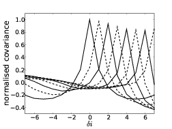 | 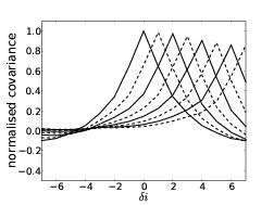 |
| (a) | (b) |
Figure 2.20: SLODAR impulse response functions in the longitudinal (a) and transverse (b) directions.
The fractional profile is scaled by the total turbulence strength which can be obtained from the tip/tilt subtracted centroid variance, this is also calculated from the fit of the SIRFs to the centroid data. The fit is used as this will provide a noiseless centroid variance [56]. r0 can be found from the centroid variance for a square aperture using [58],
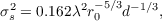 | (2.52) |
Re-arranging this and using equation 2.4,
 | (2.53) |
the integrated turbulence strength is given by,
 | (2.54) |
Figure 2.21 shows the profile recovered from the cross-covariance function show in figure 2.18.
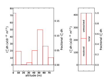
Figure 2.21: An example SLODAR profile recovered from the cross-covaraince function in figure 2.18. The panel on the right shows the resolved and unresolved integrated turbulence strength as well as the total measured integrated turbulence strength.
Shot and detector noise will increase the centroid variance introducing a bias in the centroid values. This will manifest itself in the auto-covariance function as an increased value at the central position (i.e δi = 0) and due to its random nature will act to cancel itself at all other locations. The difference between the measured centroid covariance at δi = 0 and the theoretical noiseless value from the SIRF fit will give an accurate estimate of the centroid noise. This can then be used to estimate the errors in the final profile.
As the turbulence moves across the field of view of the telescope, the corresponding phase slopes will also traverse the pupil. The covariance function of one set of centroid data with a set taken a short time later will result in a peak offset by a separation corresponding to the distance that the turbulent layer has moved in that time. In this way the cross-covariance data can be used to calculate the wind speed of each resolved layer. Figure 2.22 shows the 2D auto and cross covariance functions with an increasing temporal offset. The turbulent layer moves approximately 4 subapertures in 40 ms, which converts to approximately 5 m/s. The stationary peak at the centre is because this data has not been filtered for tube seeing. If the layer was seen in the auto-covariance but not in the cross-covariance this would mean that the turbulent layer is above the maximum resolved altitude of the instrument.
| δt = 0 ms | δt = 20 ms | δt = 40 ms |
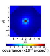 | 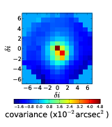 | 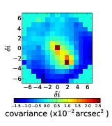 |
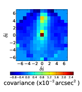 | 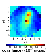 | 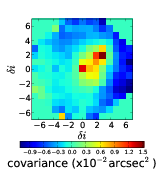 |
Figure 2.22: Example 2D auto-covariance and cross-covariance maps with increasing temporal offset, δt. By correlating one set of centroids with another set taken a time, t, later and measuring how far the correlation peak has moved we can estimate the wind speed of the turbulent layer. The top row shows the auto-covariance and the bottom row shows the cross-covariance with a temporal delay of 20 ms per frame. The data shows that on this occasion the turbulence was dominated by the surface layer. This is because the moving peaks in the cross and auto–correlation plots move in the same direction and at the same speed suggesting that it is very likely they are the same layer and there are no other obvious peaks in the auto–correlation. The residual peak in the centre is because the data has not been filtered for tube seeing.
All the above assumes that the atmospheric turbulence obeys Kolmogorov’s laws (i.e. a power spectrum with a slope of κ-11∕3). There is evidence that suggests that atmospheric does not always comply to Kolmogorov’s models (see section 2.1.2) and therefore, we might find that a different power law actually results in a better fit to the data. It is possible to calculate the SIRFs for any power law by using the non Kolmogorov power spectrum (equation 2.13). We can try to fit a number of values for β and select the one with the best fit. In this case it will no longer be r0 and Cn2(h) which we measure but ρ0 and Ωn2. This means that we will not be able to compare parameters with differing β. However, in calculating the optimum β fit we will be able to gain an insight into the mechanisms of the turbulent atmosphere.
As the mechanism which creates the surface layer turbulence and the free atmosphere turbulence are different there is no reason why the power law for the two layers should be the same. Therefore, it is possible that a different β should be used to fit each layer individually. Early results from SLODAR at SALT by R. W. Wilson show that using differential βs works particularly well.
When using SLODAR on bigger telescopes it will also be necessary to include the outer scale effects in the SIRFS. This is ignored for the small telescope case as the outer scale is likely to be much larger than the telescope and therefore subtracting the global tilt will remove any large scale aberrations.
Chapter 3
SLODAR
3.1 Introduction
3.2 The Instrument
3.3 Results
3.4 Instrument Comparisons
3.5 Discussion
3.6 Conclusion
3.1 Introduction
In this chapter a prototype of a new SLODAR instrument for atmospheric optical turbulence profiling is discussed. The instrument targets double stars with wide separations of several arc-minutes, to achieve profiling of the surface layer of optical turbulence with very high resolution in altitude (10 m or less). We describe the instrument and the results of preliminary observations at the ESO Cerro Paranal observatory.
3.2 The Instrument
The vertical resolution, δh, of the SLODAR system is given by (equation 2.50),
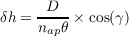 | (3.1) |
where D is the diameter of telescope aperture, nap is the number of subapertures subtended across the pupil, θ is the angular separation of the target stars and γ is the zenith angle of the observation. For more details on the SLODAR technique see section 2.8. The altitude resolution of a given SLODAR system can be improved either by increasing the number of subapertures across the pupil or by increasing the separation of the target stars. There is a limit to the number of subapertures which can be used, fundamentally determined by the photon flux. The target separation is limited by the field of view of the telescope and of the imaging detector. Targets with larger angular separations can be accommodated by employing a detector with a larger format sensor. Figure 3.1 is a diagram of the SLODAR system. The beams from the targets overlap at the lenslet array, which is in the pupil plane of the telescope. The angular separation is limited by the size of the CCD.
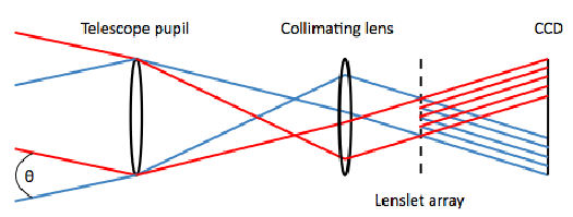
Figure 3.1: Diagram of the SL–SLODAR instrument. The red and blue lines indicate the light paths of the two stars. The lenslet array is placed in the telescope pupil plane where the beams completely overlap. The beams then separate and focus into spot patterns at different positions on the camera.
The first demonstration of the surface layer SLODAR (SL–SLODAR) instrument used a single Andor Luca EMCCD on a portable 14 inch Celestron telescope. With this instrument we could target stars with a maximum angular separation up to 12’, corresponding to a vertical resolution of 12.5 m. Figure 3.2 shows an example of the Shack–Hartmann spot patterns from this system. As we are using targets with a very large angular separation we see aberrations in the spot patterns due to the off-axis optical beams. The off-axis aberrations can be seen as larger spot separations at greater deviations from the on-axis path (i.e. towards the edge of the frame) and is therefore not simply tilt as this would result in all the spots moving by equal amounts.
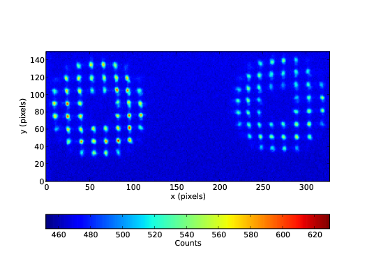
Figure 3.2: Example average SH spot pattern from a single Andor Luca EMCCD camera. The target stars had an angular separation of 12’. The off-axis aberrations can be seen in the spot patterns.
The centroid position is calculated relative to the average position of the spot. It is therefore insensitive to static aberrations unless the aberration results in a variable spot motion for the same local tilt in different areas of the pupil. This can be diagnosed by examining the time averaged centroid variance as a function of position in the pupil. In an ideal situation the time averaged centroid variance in every subaperture will be the same, the value of which will correspond to the seeing. If the aberration was causing larger spot motions then the centroid variance would also be larger. Figure 3.3 shows a 2D map of the mean centroid variance for centroid motion in the direction joining the two stars and orthogonal to it. There is no gradient in variance across the pupil suggesting that aberrations of this scale do not effect the centroiding process.
The edge subapertures do have a larger than average variance. This is probably due to mis-alignment of the optics so that the edge subapertures are vignetted and not fully illuminated. The pupil is not exactly sampled by the 8 × 8 subapertures.
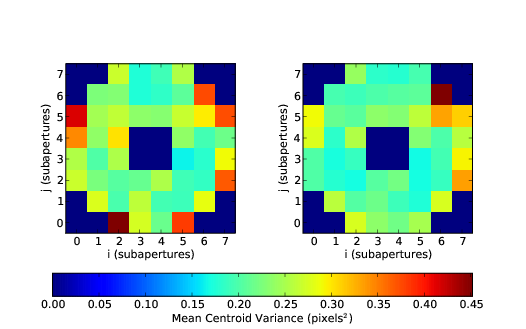 |
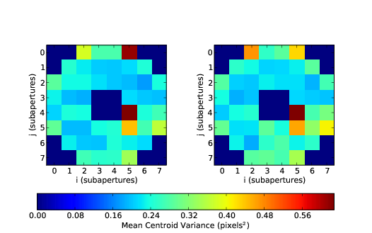 |
Figure 3.3: Time averaged centroid variance for the single camera wavefront sensor for centroid motion in the direction joining the two stars (top panel) and orthogonal to it (lower panel). The subapertures with anomalously high variances indicate a mis-alignment of the optics. The mean centroid variance value is 0.20±0.06 pixels2.
Although the large format CCD used here does allow for impressive results this method typically implies greatly increased detector readout times and still has a limit to the star separation, albeit a larger one. Windowing of the CCD has been used to reduce the read out times however the spot patterns are located at the edge of frame and so it is not possible to use any stars with greater separations to achieve higher vertical resolution. Instead, we have modified the system to include a reflective wedge to divert the light from the two target stars into separate, synchronized, wavefront sensors (figure 3.4). The target separation is now limited only by the telescope field of view and can be tuned by moving the wedge along the optical axis. With this modification targets with an angular separation of ~16′ and a 0.4 m telescope have been used to yield a vertical resolution of less than 10 m. Richard Wilson is responsible for the optical design of this instrument and Timothy Butterley for the impulse response function fitting. The author was responsible for the data collection, the rest of the data reduction and all of the data analysis.
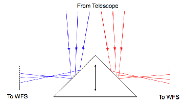
Figure 3.4: SL–SLODAR employs a reflective wedge to divert the light from the two target stars into separate wavefront sensors. Targets with very large angular separations can then be observed. The wedge is mounted on a single axis stage so that the correct angular separation can be selected for a given target.
The optics of the SLODAR system are chosen and aligned carefully to ensure that the correct spot size and motion can be measured. Figure 3.5 is a diagram of the optics and dimensions of the SL–SLODAR system at Paranal on the 16 inch Meade telescope.
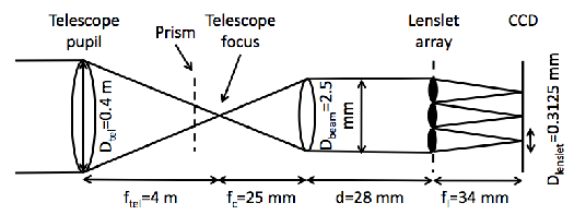
Figure 3.5: Diagram of SL–SLODAR optics and dimensions. The dashed line indicates the position of the reflective wedge where the light will be folded into two identical arms.
The lenslet array has a pitch, Dlenslet, of 0.3125 mm therefore, if we want 8 × 8 subapertures the beam diameter, Dbeam, must be,
 | (3.2) |
This constrains the collimator to have a focal length, fcol, of,
 | (3.3) |
where f∕# is the f number of the telescope and for the Meade this is 10. The diameter of the collimator is not important but should be considerably larger than the beam diameter to minimise aberrations on off-axis beams. The pixel scale of the telescope is given by,
 | (3.4) |
The pixel scale on the CCD can be found by multiplying this by the magnification of the system,
 | (3.5) |
where flenslet is the focal length of the lenslet array. The camera is set to bin the pixels 2 × 2, each of which has a diameter of Dpix = 10μm, therefore the final CCD pixel scale will be 38 × Dpix × 2 = 0.76′′ pixel-1.
In the prototype SL–SLODAR instrument, each channel comprises a Shack-Hartmann wavefront sensor, deploying 8 × 8 sub-apertures across the telescope pupil, and equipped with an Andor Luca EM-CCD camera. The cameras have a peak quantum efficiency of approximately 50% and effectively zero read noise whilst running with a frame rate of approximately 60 Hz and an exposure time between 2 and 5 ms. The centroid slopes can be temporally filtered at 1 Hz to remove the tube seeing. CCD exposures were synchronized via an external electronic trigger signal. A photograph of the instrument identifying the components is shown in figure 3.6. The instrument was mounted on a 0.4 m Meade telescope, as shown in figure 3.7.
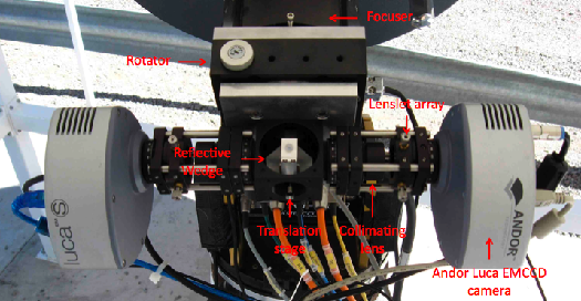
Figure 3.6: Photograph of the SL–SLODAR identifying the optical components.
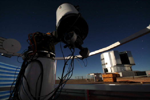
Figure 3.7: Photograph of the SL–SLODAR on the 16 inch Meade telescope at Paranal.
Figure 3.8 shows an example of the time averaged Shack–Hartmann spot patterns from the modified system. The image shows considerably less windshake than in figure 3.2. This is because the Meade telescope on the Astelco mount is a much more rigid structure than the commercial Celestron telescope mount.
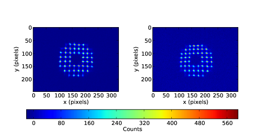
Figure 3.8: Example SH spot pattern from two single Andor Luca EMCCD cameras. The target stars had an angular separation of 16’. There are still off-axis aberrations but very little windshake.
Figure 3.9 shows the time averaged 2D centroid variance maps for the modified system. The centroid variance is essentially constant with pupil position suggesting that the optics are all well aligned.
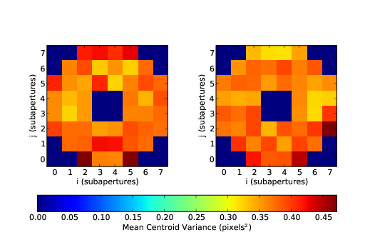 |
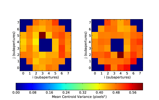 |
Figure 3.9: Time averaged centroid variance for two cameras for centroid motion in the direction joining the two stars (top panel) and orthogonal to it (lower panel). The centroid variance is constant across the pupil indicating that the optics are well aligned and that the aberrations do not effect the instrument. The mean centroid variance is 0.44±0.03 pixels2.
3.3 Results
The prototype SL–SLODAR instrument was operated at Cerro Paranal for a total of 17 nights in February 2009 and April 2009. An example turbulence profile sequence is shown in figure 3.10. The altitude resolution changes gradually as a function of time, because the vertical resolution of SLODAR is scaled by the air mass of the target (equation 2.50). There are also discrete changes in resolution due to changes of the target star.
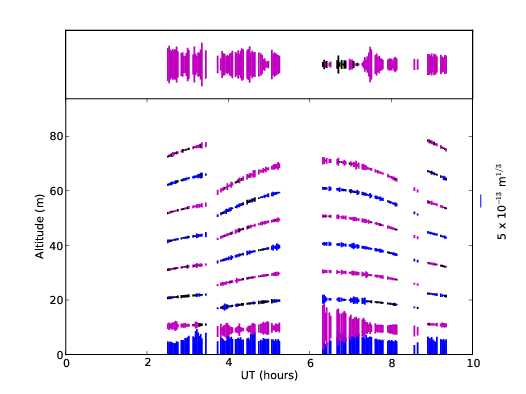
Figure 3.10: Example SL–SLODAR profile sequence for the night of 9th April 2009. The thickness of the trace at each point indicates the strength of the turbulence at that altitude, with alternate bins coloured blue and purple for clarity. The trace in the upper box shows the integrated strength of the unresolved turbulence at higher altitudes. Black lines indicate negative values: the fit of turbulence strength to the data does not enforce positivity, so that small negative values are expected as a result of noise. Note the systematic change in resolution of SLODAR as the elevation of the target stars varies. Step changes indicate a change of target.
Figure 3.11 shows the histogram of vertical resolution values. The median resolution is 9.3 m with maximum and minimum values of 11.2 m and 5.8 m respectively.
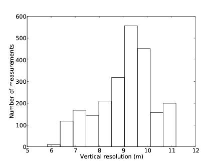
Figure 3.11: The SLODAR vertical resolution changes depending on the angular separation and the elevation of the targets. The histogram shows resolution achieved with SL–SLODAR over the 17 nights in January and April 2009.
Figure 3.12 is a plot of the median profile measured for Paranal over 17 nights. Since the resolution changes with the air mass of the target, the median profile was calculated by re-binning the data assuming a uniform distribution in each bin. The median profile is not representative of any particular profile and is shown only for completeness. The median profile shows a substantial surface layer contribution, concentrated near the ground and with a scale height of 11 m. The subplot on the right shows the integrated Cn2(h) value for the surface layer and the higher altitude atmosphere (above the limit of direct profiling), as well as the median total turbulence strength (integral over all altitudes). Note that the two subplots have different vertical scales.
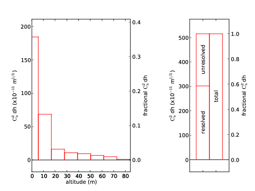
Figure 3.12: The median surface layer profile for data acquired on 17 nights in February 2009 and April 2009, at Cerro Paranal, Chile. The subplot on the left shows the surface layer profile which has a strong boundary layer and a decay height of approximately 11 m. The subplot on the right shows the integrated surface layer (resolved) turbulence and the integrated (unresolved) contribution from higher altitudes, and also the median total turbulence strength for all altitudes.
3.4 Instrument Comparisons
In order to validate the results for SL–SLODAR we compare with contemporaneous data from an independent turbulence monitor, the combined MASS–DIMM instrument of the VLT automated site monitor (ASM) situated at Paranal.
Figure 3.13 plots the seeing value at Paranal for the night of 9th April 2009 as estimated by the DIMM (Differential Image Motion Monitor [26]). The DIMM is a well calibrated and tested instrument capable of accurately measuring the integrated optical turbulence strength for the line of sight to its target star. The seeing is corrected for airmass to estimate the seeing at the zenith. The plot also shows the total seeing determined from SL–SLODAR on the same night. The DIMM is located on a tower approximately 6 m higher than SL–SLODAR. Hence we may expect the SL–SLODAR values to be systematically larger than for the DIMM if there is significant turbulence strength in the first 6m altitude. By removing the first SL–SLODAR bin, the two seeing estimates are more closely matched in terms of air mass. The median vertical resolution for this night was 9.6 m (9.4 m for all data). The SL–SLODAR instrument is mounted at approximately 2 m so that if we subtract the first SL–SLODAR bin (which is centred at the SLODAR telescope) we obtain a seeing estimate for the whole atmosphere excluding the first ~6 m. This is also shown on figure 3.13, and a greatly improved agreement with the DIMM is apparent.
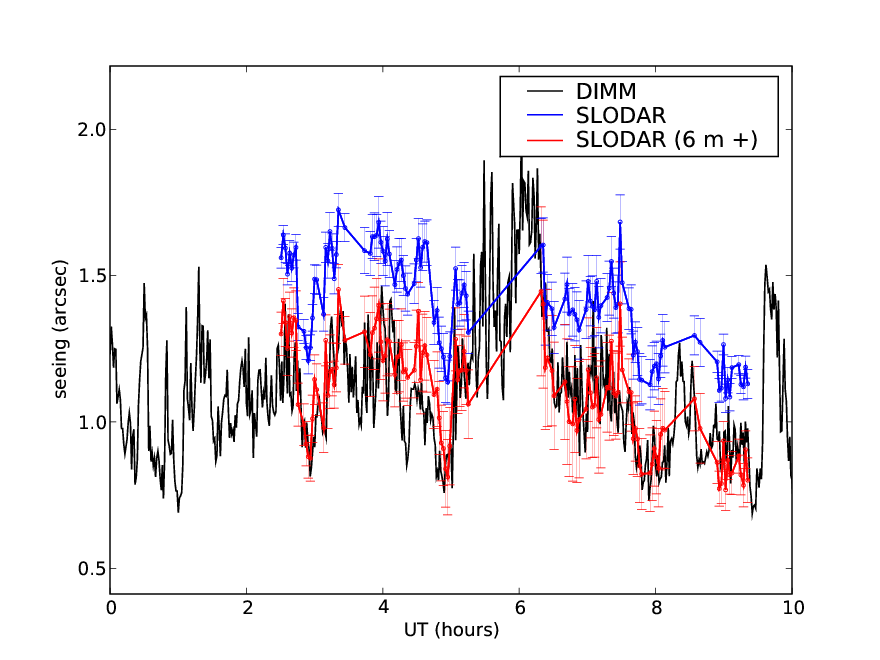
Figure 3.13: Comparison of the seeing values (corresponding to the integrated turbulence strength for the whole atmosphere) for SL–SLODAR and DIMM for the night of 9th April 2009. The black line shows the seeing from the Paranal DIMM site monitor and the blue line is the seeing as calculated by SL–SLODAR. The red line is the seeing for the SL–SLODAR 6m+ calculated by subtracting the first bin to give an estimate of the seeing from 6 m, to match the altitude of the DIMM.
Figure 3.14 compares the SL–SLODAR and the DIMM integrated Cn2 values for the 17 nights of observations. SL–SLODAR has been corrected for the altitude difference. The plot shows a correlation of 0.8 between the seeing measured by the two instruments. Some scatter is expected due to the spatial separation of the two instruments and the fact that the instruments monitor different targets through different volumes of the atmosphere. The median integrated Cn2(h) value for the DIMM is 522 × 10-15 ± 29 × 10-15m1∕3 compared to the median for SL–SLODAR (6m+) of 533 × 10-15 ± 21 × 10-15m1∕3. The two instruments agree within the limits of the estimated errors.
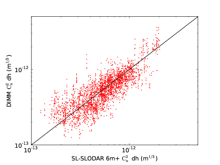
Figure 3.14: Cn2 comparison between SL–SLODAR above 6 m and DIMM. The correlation coefficient is 0.8 but there is significant scatter as expected due to the spatial separation of the instruments and their use of different target stars.
Figure 3.15 compares the integrated turbulence strength for the directly resolved SL–SLODAR altitudes (again excluding the first bin) to contemporaneous measures of the turbulence below 250m altitude provided by the MASS–DIMM instrument for the 2009 data. The MASS (Multi-Aperture Scintillation Sensor [53]) recovers the turbulence profile from measurements of the scintillation indices for a set of concentric ring apertures. The MASS is not sensitive to turbulence below an altitude of approximately 250m. However when combined in operation with the DIMM, which senses the integrated turbulence for all altitudes, the total turbulence in the first 250m altitude can be found by differencing.
Here we compare the integrated turbulence from ~6 m up to the maximum altitudes resolved by the SL–SLODAR (altitudes up to approx. 80m) with the surface layer estimate from the MASS–DIMM (below approx. 250m). There is a discrepancy in the maximum altitude included in each case, since the altitude range 80 to 250 m is not directly profiled by the SL–SLODAR. However, previous observations with the original SLODAR instrument at Paranal, which profiled with lower resolution to an altitude of approx. 1km, showed that the turbulence strength is typically weak at these altitudes [7]. Hence we may expect the SL–SLODAR integral to be comparable with the MASS–DIMM surface layer measure in most cases. From figure 3.15 we see that this is broadly the case, although again there is substantial scatter due to line–of–sight differences. There were also a significant number of occasions on which the SL–SLODAR integral was lower than the MASS–DIMM value, probably due to instances of stronger than average turbulence strength in the 80–250m zone. The median turbulence strength was 130 × 10-15 ± 5 × 10-15m1∕3 and 223 × 10-15 ± 13 × 10-15m1∕3 for SL–SLODAR and MASS–DIMM respectively.
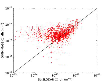
Figure 3.15: Comparison of the integrated turbulence strength for the surface layer between SL–SLODAR and MASS–DIMM.
SL–SLODAR has also been compared with LuSci. Figure 3.16 shows the integrated turbulence strength as measured concurrently by the two instruments over 16 nights in February 2009 and April 2009. The LuSci integrals were calculated from 2 m to the maximum SLODAR altitude at the time of observation. The median SL–SLODAR measurement was 125 × 10-15m1∕3 and LuSci recorded 42 × 10-15m1∕3. Although there is obviously a systematic difference between the instruments the correlation coefficient is 0.71.
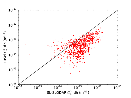
Figure 3.16: Comparison of the integrated turbulence strength for the surface layer as measured by SL–SLODAR and LuSci. The LuSci measurements were integrated from 2 m to the SL–SLODAR maximum height.
Figure 3.17 shows a comparison of the integrated turbulence strength for the surface layer as measured by DIMM-MASS and LuSci. The median values are 250 × 10-15m1∕3 and 51 × 10-15m1∕3 respectively.
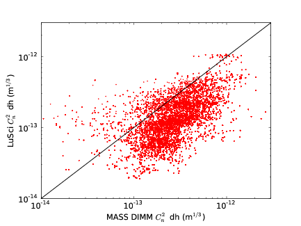
Figure 3.17: Comparison of the integrated turbulence strength for the surface layer as measured by LuSci and DIMM – MASS. The LuSci integrals are calculated between 6 m and 250 m.
Both of these comparisons show a large systematic discrepancy which is explained by Tokovinin et al. [50] by the fact that the surface layer at Paranal is tilted. Paranal observatory is located on a plateau with steep sides to the desert floor. The prevailing wind comes from the north and is likely to generate turbulence as it is pushed up by the plateau. SL–SLODAR and the MASS–DIMM predominantly point south towards the celestial pole, however, LuSci profiles the turbulence north of the plateau towards the moon.
3.5 Discussion
The example shown from 9th April 2009 is an interesting one as it shows events at the ground as well as in the second bin and above in the unresolved bin. Figure 3.18 is an example of slow variability in a strong surface layer with very little at other altitudes. The bottom panel shows a comparison of the seeing angle measured by SL–SLODAR, SL–SLODAR 6 m+ and the DIMM. The difference between SL–SLODAR and SL–SLODAR 6 m+ is large demonstrating the strength of this extremely thin surface layer.
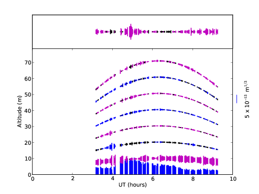
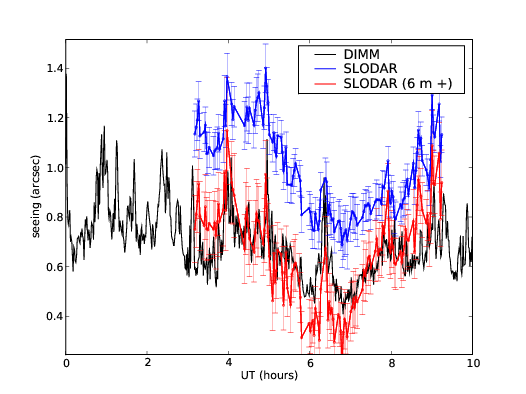
Figure 3.18: Often the seeing is dominated by the surface layer. In this example we observe a very strong slowly varying surface layer and a generally weak high layer. The lower panel shows the total seeing as a function of time for the SL–SLODAR, SL–SLODAR 6 m+ and the DIMM.
We have also observed occasions when the surface layer has been extremely weak and the seeing has been dominated by unresolved turbulence (figure 3.19). SLODAR is unable to identify the altitude of this turbulence but contemporaneous measurements from MASS (figure 3.20) show strong turbulence in the 2nd and 3rd bin corresponding to bins centred at 1 and 2 km. These might be two layers or more likely (due to the strong correlation) a single turbulent layer which has been split between the MASS bins due to the overlapping response functions.
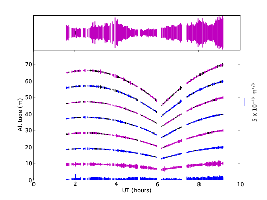
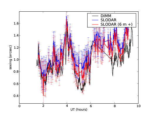
Figure 3.19: An example of a night where the surface layer was particularly quiet. In this case the seeing was dominated by the unresolved turbulence. Figure 3.20 shows the MASS profile from the same night and reveals a strong layer at approximately 1.5 km.
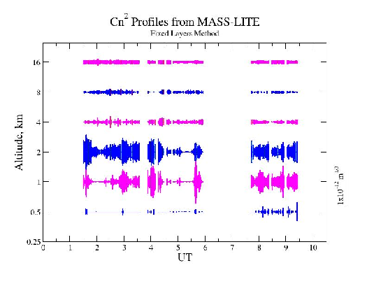
Figure 3.20: The MASS profile from the same night as figure 3.19 shows a strong layer at approximately 1.5 km. The data could indicate two layers, however the strong correlation in structure suggests that it is actually a single layer located on the boundary of the two over lapping response functions of the MASS. From Paranal data archives.
So far all the examples have only shown structure in the first two resolved bins. Figure 3.21 shows a night with activity at all altitudes.
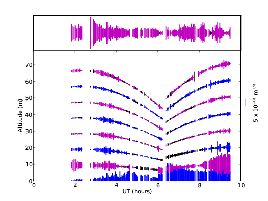
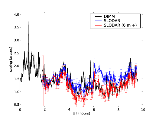
Figure 3.21: On this occasion there is turbulent activity recorded at all altitudes. This is indicative of a night with particularly bad seeing. At approximately 0700 the first bin measures a strong rise in turbulence strength. This is not seen by the DIMM and is demonstrated by the difference between the SL–SLODAR total (blue line) and the SL–SLODAR 6 m+ measurement (red line).
We are currently constructing a robotic version of SL–SLODAR that will be permanently based at Paranal providing vital information on the surface layer over a long period of time. Until this is complete we only have data from a limited number of nights from the prototype. We do not yet have enough data to present a statistically significant study on the surface layer at Paranal but it is possible to comment on the results from the prototype.
It has been observed that the seeing at Paranal as measured by the DIMM is often considerably worse than the seeing measured by the UTs. The DIMM median seeing in 2009 was approximately 1.1′′ compared to the median value from Isaac and FORS2 which was approximately 0.65′′. It is possible that this difference could be explained by selection or outer scale effects. If the outer scale is of the same order as the size of the telescope the low order modes will be averaged out resulting in better image quality. However, Sarazin et al. [59] noted that the DIMM seeing has been steadily deteriorating since construction of the UTs. Archives show that the seeing as measured by the DIMM has degraded from a median value of ~0.65′′ in 1990 to ~1.1′′ in 2009. However, the seeing as measured by Isaac and FORS2 has remained virtually constant during this time. Sarazin suggests that this difference is due to changes in the prevailing surface layer conditions. For this to be the case they hypothesise that the surface layer at Paranal must be extremely thin so that it will effect the DIMM but not the UTs. The data from SL–SLODAR supports this hypothesis showing a very strong and thin surface layer with nearly 20% of the total turbulence between the DIMM height (6 m) and the UT dome height (30 m) with a scale height of 11 m.
3.6 Conclusion
We have developed a modified SLODAR instrument which can profile the surface turbulent layer with high resolution in altitude (less than 10 m). This was achieved by employing separate wavefront sensor channels for each of the target stars, to allow for greater separations and therefore a higher resolution. Early data collected at Paranal are consistent with contemporaneous DIMM and MASS measurements. Comparisons with LuSci demonstrate a systematic error which is also observed in the LuSci / MASS–DIMM comparison. This could be explained by the fact that SL–SLODAR and the MASS–DIMM predominantly point south over the plateau and LuSci points north over the edge, suggesting that the turbulence profile of the surface layer is directional. More data is required to make any statistical generalisation about the surface layer at Paranal. We are currently working towards increased automation of the SL–SLODAR system to this end.
The information from SL–SLODAR would also be valuable at the site testing, selection and characterisation stage for future observatories as it would allow estimations of the seeing expected from telescopes at heights other than the DIMM platform. It will also be possible to estimate the seeing in altitude ranges above the telescope in order to model the performance of AO systems.
Chapter 4
Adaptive Pupil Masking
4.1 Introduction
4.2 Simulation
4.3 Threshold Selection
4.4 High contrast imaging
4.5 Conclusions
4.1 Introduction
The turbulent atmosphere causes phase variations across a wavefront propagating from an astronomical object to a ground based telescope. It is well known that these distortions degrade the imaging performance of the telescope and the whole field of adaptive optics (AO) has been developed to ameliorate these distortions. However, no AO system is perfect and the partially corrected point spread function (PSF) from a typical AO system consists of a diffraction limited core sitting on top of a much broader halo. The short exposure halo is made up from speckles which are averaged in a long exposure to produce a large (in angular extent) low level plateau which can limit the achievable signal to noise ratio of the detection of faint objects around bright stars.
Here we describe a method to reduce residual speckles in an adaptive optics system and which add to the halo of the point spread function (PSF). The halo is particularly problematic in astronomical applications involving the detection of faint companions. Areas of the pupil are selected where the residual wavefront aberrations are large and these are masked using a spatial light modulator. The method is also suitable for smaller telescopes without adaptive optics as a relatively simple method to increase the resolution of the telescope. We describe the principle of the technique and show simulation results.
Areas of the wavefront whose phase error is larger than some threshold value are completely blocked. If we mask some of the aperture then we are clearly reducing the throughput of the system, but we are also blocking the areas of the wavefront which tend to produce the halo rather than the central core of the PSF. We propose to use an amplitude modulating spatial light modulator (SLM) as the active element. We show that blocking areas of the pupil can lead to both a reduction in the halo intensity and an increase in the central intensity.
There are other methods for improving the performance of telescopes which are related to adaptive pupil masking. In a binary adaptive optics system [60] areas of the pupil which are more than half a wave out of phase (modulo 2π) have a correction of π added to them. The basic philosophy behind binary AO is that all the parts of the wavefront which have a phase error of less than π are adding approximately constructively at the telescope focus – and therefore should be left unchanged. Areas of the wavefront which have an error of greater than π are adding destructively at the telescope focus and therefore if a correction of π is added then there will be a dramatic improvement of imaging performance. The proposed method of adaptive pupil masking is similar, except here we completely remove areas of the pupil with large phase errors, plus the criterium for masking is not necessarily a phase error of π. These are important differences as it means that this method is more suitable for use as an addition after a conventional AO system and before coronagraphic techniques – rather than binary AO which was proposed as a simple approach to full AO.
The adaptive pupil mask is also a variation on the Lucky Imaging-type techniques. This was first proposed by Fried [61] and consists of recording many short exposure images without adaptive optics. A fraction of these images are selected, according to their quality, and are co-added to produce impressive results [62]. The probability, P, of observing a ‘lucky image’ (an image with phase variance less than 1 rad2 as defined by Fried) can be calculated using ([61]),
![[ ]
( D )2
P ≈ 5.6exp - 0.1557 r-
0](/wp-content/uploads/sites/167/2021/04/thesis134x.png) | (4.1) |
for D∕r0 > 3.5, where D is the diameter of the telescope pupil and r0 is the Fried parameter. As the telescope size increases the probability of observing a lucky image decreases with a strong function of D∕r0 which makes the method ideal for small telescopes but for larger telescopes the probability becomes so high that the method is unusable. A low order AO system increases the probability and has been demonstrated on larger telescopes [63]. Here we present a development of the standard lucky imaging method to increase its efficiency on telescopes of all sizes. Instead of temporally filtering the wavefront we spatially filter. This is similar to the work by Morossi et al. [64] who spatially select the best subapertures on a large telescope and co-add them in order to improve the resolution in the visible with AO systems configured for the IR. However, we do not co-add instead we simply block the subapertures conserving the full resolution of the telescope.
The adaptive pupil mask could be deployed on any telescope, for example a small telescope without AO or a larger telescope with AO. For a telescope with AO the threshold can be set so that the piston cutoff is smaller than the residual piston after the AO correction in order to reduce the phase variance further. Small or medium sized telescopes are often left uncorrected due to the cost in pounds and complexity of a full AO system. The adaptive pupil mask could be used to improve the performance of these telescopes for a fraction of the cost. The reduced phase variance will result in reduced halo, increased peak intensity and reduced full width at half maximum (FWHM) of the PSF which will be useful in many areas of astronomy. For example it could be beneficial for multi-object spectrographs as the reduced FWHM will minimise the cross talk between the spectrograph channels. The example used in this paper to quantify the possible improvements is the detection of faint companions. We show that the signal to noise ratio is significantly improved by using the adaptive pupil mask. It should be noted that although we use the example of faint companion detection it is unlikely that the technique will be useful for terrestrial exoplanet detection. This is because the detection of extrasolar planets requires extremely low residual phase variance in order to have sensible exposure times and when we obtain this using extreme AO other factors then start to become significant. Quasi static speckles ([65], [66], [67] and many others) appear due to the flaws in the optical surfaces and setup. These speckles are not static enough to be subtracted and not variable enough to average out. The temporal and spatial statistics of these speckles will be changed by the adaptive pupil mask changing the shape of the telescope pupil throughout an observation meaning that angular differential imaging [68], as used by Marois et al. [1] in the first direct imaging of an extra solar planet, will no longer work. Scintillation is also a fundamental problem for the direct detection of extrasolar planets [69], [70] as this will alter the pupil function which will change the PSF. This was not included in the simulations or theoretical work as the effect is only significant when the phase variance is near to zero which we did not approach in the simulations.
In the following sections we present results of a simulation of the technique and a theoretical analysis which explains the critical threshold values.
4.2 Simulation
Using the AO simulation framework developed at Durham University [44] we have implemented and executed a full AO simulation including the adaptive pupil mask. The simulation consists of a single turbulent layer with a Fried parameter, r0, of 0.15 m and a wavelength, λ, of 500 nm. The location of the turbulence is not important here as the simulation assumes geometric wave propagation. The phase aberrations add linearly and so it is only the integrated turbulence strength which is important. This assumes that the WFS subapertures are larger than the spatial correlation scale of any scintillation and so the near field approximation can be used. The phase screen is randomly evolving and is blown across the pupil of the telescope at 5 m/s. The segmented deformable mirror is modeled on the Durham ELECTRA mirror [71] allowing three degrees of freedom for each segment (piston, tip and tilt) with either 8×8 or 16×16 subapertures. The phase is measured via a Shack-Hartmann wavefront sensor (WFS) and a successive over-relaxation reconstruction algorithm estimates the phase map and passes the data to the mirror and the adaptive pupil mask. The mask is placed after the mirror and WFS pickoff in the pupil plane. The adaptive pupil mask will have the same geometry as the WFS (either 8×8 or 16×16 in this case). Ideally the subapertures will be a similar size to r0 to achieve the optimum performance although this is not necessary. The pupil mask blocks the subapertures which have a reconstructed piston greater than a threshold value and updates at the same rate as the deformable mirror (every 5 ms). The threshold value chosen will depend on the strength of the turbulence in the atmosphere and the requirements of the user and will be discussed in section 4.3. Figure 4.1 shows the data flow of the simulation and the location of the pupil mask within the optical train.

Figure 4.1: Block diagram for the adaptive pupil mask system. The mask is positioned in the pupil plane of the telescope after the deformable mirror (DM) and after the wavefront sensor (WFS) pickoff.
The examples below were chosen to show the mask in two different regimes. (1) The small telescope scenario (1 m without AO, with 8×8 WFS) and (2) the large telescope scenario (8 m with 16×16 AO). By blocking subapertures with a large instantaneous phase excursion the wavefront will be flatter. The result of which is a reduced PSF halo and an increased peak intensity. The extent of the PSF improvement is dependent on the wavefront variance after the blocking and so the the lower the wavefront phase threshold we choose to block the greater the fraction of the pupil is removed and the flatter the wavefront becomes. However, blocking the pupil will also reduce the total intensity of the PSF and modify the diffraction pattern. The optimum threshold is a balance between these two effects and can be found from plots of the full width at half maximum (FWHM) of the PSF (figure 4.2) and the peak intensity of the PSF (figure 4.3) as a function of the threshold value.
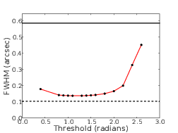 | 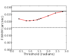 |
| (a) | (b) |
Figure 4.2: Simulation results showing how the FWHM of the PSF is modified by the adaptive pupil mask. All areas of the pupil which have a phase error greater than the threshold (either positive or negative) are blocked. The plots show the FWHM for (a) a 1 m class telescope and (b) an 8 m telescope with AO. The solid horizontal black line at the top of the plot shows the FWHM without the adaptive pupil mask and the dashed line at the bottom shows the FWHM for a perfect system with no aberrations. For a large threshold only a small fraction of the pupil is blocked and there is little change of the PSF. As the threshold is reduced more of the pupil is blocked, the resulting wavefront is flatter and the FWHM is reduced. If the threshold is too low we block a large fraction of the pupil broadening the diffraction pattern due to the low fill factor of the pupil.
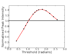 | 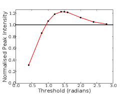 |
| (a) | (b) |
Figure 4.3: Simulation results showing how the peak intensity of the PSF is modified by the adaptive pupil mask. (a) shows the peak intensity for the 1 m telescope without AO and (b) for the 8 m telescope with AO. The solid black line indicates the peak intensity of the PSF with no blocking. For low threshold values large fractions of the pupil are blocked and so the total intensity is also reduced by a large amount. For high threshold values the effect is negligible, but there is an intermediate value where the peak intensity is increased. The intensity is normalised to the peak value without a pupil mask.
To quantify the improvements for a specific case in both of the following examples the threshold is chosen to maximise the peak intensity. The first example, figure 4.4, shows a 3D plot of the PSF from a 1 m telescope without a deformable mirror but using a WFS with 8×8 subapertures and the threshold was chosen to be ± 1.8 radians. The intensity of the PSF is increased by 40 % and the FWHM is reduced from 0.58′′ to 0.16′′ with the diffraction limited FWHM being just 0.13′′. On average 42 % of the pupil was blocked.
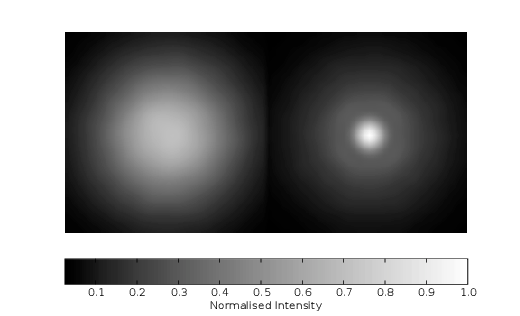 |
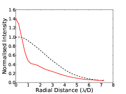 |
Figure 4.4: Example PSF from a 1 m telescope without AO with r0 = 0.15 m. On the top left is the original PSF from the telescope with no AO and on the top right is the PSF with no AO but using the adaptive pupil mask with a threshold value of ± 1.8 radians. The bottom plot shows the radial intensity profiles of the two PSFs. The black dashed line is the original intensity pattern and the red line is the modified radial profile. The modified intensity is 40 % higher and the FWHM 4 times smaller than the original PSF.
Figure 4.5 is a 3D plot of the PSF from an 8 m telescope with a 16×16 AO system. The peak intensity of the PSF is increased by a factor 0.23 and the FWHM is reduced from 0.022′′ to 0.018′′ with the diffraction limited FWHM being 0.016′′. The threshold was ± 1.4 radians and on average 19 % of the pupil was blocked.
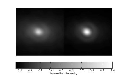 |
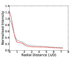 |
Figure 4.5: Example PSF from an 8 m telescope equipped with a 16×16 AO system with r0 = 0.15 m. On the top left is the original PSF from the telescope and on the top right is the PSF with AO and the adaptive pupil mask and a threshold value of ± 1.4 radians. The bottom plot shows the radial intensity profiles of the two PSFs. The black dashed line is the original intensity pattern and the red line is the modified radial profile. The modified intensity is 23 % higher and the FWHM is reduced from 0.022 ” to 0.018 ”. As the fraction of the light in the core has been increased the halo component is seen to be reduced.
The advantage of this technique can be quantified by considering the case of the detection of faint companions. As a consequence of the reduced fraction of energy in the PSF halo the background count from the parent star at the position of the companion will be lower. Combining this with the increased peak intensity results in an improved contrast ratio which equates to either a higher signal to noise ratio (SNR) or a reduced exposure time to obtain a target SNR. As the simulation were all run for a simulation time of 100 seconds the results presented here are in terms of the possible gains in SNR. Figure 4.6 shows the SNR as a function of the threshold assuming no sky background and a detector with 100 % quantum efficency. The threshold for maximum SNR is different to the optimum threshold for peak intensity as it is a balance between maximising the peak intensity and minimising the FWHM.
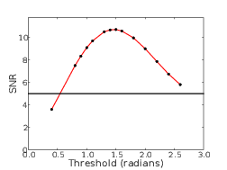 | 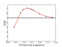 |
| (a) | (b) |
Figure 4.6: SNR obtained as a function of threshold for observing a faint companion at 2λ∕D and δm = 7.7 with a D = 1 m telescope (a) and δm = 11.7 with a D = 8 m telescope (b). The solid black line shows the SNR for the un-masked system.
The simulation results are shown in table 4.1. The magnitude difference in each case is chosen so that the SNR after 100 s is 5 and the angular separation of the companions is 2λ∕D. For a 1 m telescope this corresponds to a magnitude difference of 7.7 and a difference of 11.7 with an 8 m telescope. The noise terms in the SNR ratio include the shot noise from the star at the location of the companion and the shot noise due to the signal from the companion. The exposure time is assumed to be long enough to average out PSF speckle and therefore speckle noise is not included. The adaptive pupil mask substantially increases the SNR in both cases, doubling it to 10.5 for a 1 m telescope and increasing it to 7.1 for the 8 m telescope. A four quadrant phase mask (FQPM) coronagraph [72] can be used to further increase the SNR for faint companion detection by reducing the light from the parent star (we stress that our proposed technique may not be suitable for detecting terrestrial exoplanets – but a coronagraph can be useful in general for detecting faint companions). The FQPM coronagraph is sensitive to pupil geometry [73] and so the adaptive pupil mask will mean that the coronagraph can not operate as effectively as it could. But the reduced wavefront variance after the pupil mask will also mean that the FQPM coronagraph will be more efficient [74]. The simulation results show that the reduced phase variance outweighs the effects of the changing pupil geometry and that the coronagraph actually works better after the adaptive pupil mask and so the combination of the pupil mask and coronograph results in an SNR of 10.6, twice the original value. Figure 4.7 shows radial cuts of the PSF after the coronagraph with and without the pupil mask.
| SNR | ||||||
| Tel Diam (m) | δ Mag | AO | control | APM | FQPM | APM + FQPM |
| 1 | 7.7 | no | 5 | 10.5 | – | – |
| 8 | 11.7 | yes | 5 | 7.1 | 6.6 | 10.6 |
Table 4.1: Simulation results for a combination of different telescope diameters and instruments to show the achievable SNR with each system. The target separation was chosen to be 2λ∕D and the magnitude difference (δ Mag) of the binary system was selected so that the signal to noise ration (SNR) of the system without the mask (control) was 5. The adaptive pupil mask (APM) can then increase the SNR dramatically. For the 8 m telescope the SNR with a four quadrant phase mask coronagraph (FQPM) and the combination of the APM and FQPM is shown.
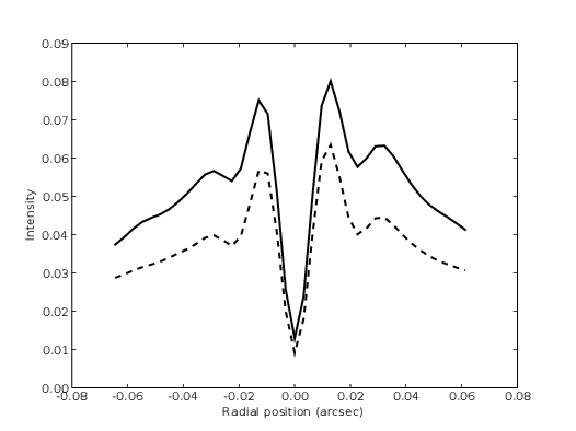
Figure 4.7: Radial cut of PSF after the four-quadrant phase mask coronagraph. The solid lines are the PSFs after AO correction and the four quadrant phase mask coronagraph and the dotted lines are the PSFs after AO, pupil masking and the four quadrant phase mask coronagraph. The extinction is not as good as the diffraction limited case as the coronagraph is very sensitive to residual tilt. The pupil mask will reduce some of the residual wavefront error and hence result in greater extinction.
4.3 Threshold Selection
It is important to calculate the optimum phase threshold for the system. This could be done in real time on sky by a trial and improvement strategy however it would be useful to be able to calculate the optimum threshold from measurements of the immediate seeing. In order to do this an analysis of the performance of the mask as a function of wavefront variance is required. The analysis will also help to explain the idea and the limitations of pupil masking.
The analysis treats the atmosphere and the telescope as separate spatial filters. For pupil masking and AO correction we assume that the wavefront correction takes place before the telescope accepts the wavefront. In doing this we can de-couple the telescope and atmospheric effects. The point spread function can be calculated by (from equation 2.25),
![( I′)
P SF = (F [M TF atmos × M TFtel])× TI--
T](/wp-content/uploads/sites/167/2021/04/thesis147x.png) | (4.2) |
where denotes the Fourier transform, MTFatmos is the atmospheric modulation transfer function, MTFtel is the telescope modulation transfer function and I′T∕IT is the ratio of the modified total intensity, I′T, to the original total intensity, IT, and is equal to the fraction of the pupil which is not blocked by the mask. In chapter 2 we derived equations for the phase structure function for uncorrected and partially corrected wavefronts. Fried [17] calculated the phase structure function for uncorrected wavefronts to be,
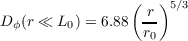 | (4.3) |
and for large r,
 | (4.4) |
where L0 is the outer scale of the turbulence and σϕ2 is the phase variance. At separations greater than the outer scale the structure function converges to a constant. For partially corrected wavefronts we use a filter function to remove the low order modes, as described in chapter 2. This filter is derived by Greenwood et al. [28] as,
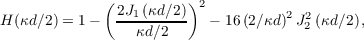 | (4.5) |
and using equation 2.33 the phase structure function can be written as,
![∫ ∞
Dϕ,AO (x) = 45.8σ2ϕ [1- J0(ux )]H (u∕2)u-8∕3du.
0](/wp-content/uploads/sites/167/2021/04/thesis151x.png) | (4.6) |
Gaussian statistics can be used to describe independent atmospherically induced fluctuations in the phase of a wavefront [14]. The atmospheric turbulence induced phase aberrations are fractal, they are self similar on all scales. Therefore if we remove the low order modes with an AO system the residual phase fluctuations are still Gaussian in nature. So, whether or not the adaptive pupil mask is used in conjunction with an AO system the piston distribution (P(ϕ)) will be a Gaussian with variance, σϕ2. In the case that the phase variance is large the piston distribution will be two π phase wrapped. The adaptive mask will block the subapertures with the largest phase, truncating the Gaussian at +/- T, where T is the threshold piston value. The variance will therefore be reduced to,
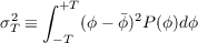 | (4.7) |
where ϕ is the mean piston of the wavefront. We can now plot the residual variance after the mask as a function of the initial variance entering the adaptive mask and the threshold chosen (figure 4.8 (a)). By knowing the input wavefront variance and choosing a threshold value we can select the resultant variance we require. However, it is important to take account of the changing diffraction limited PSF and in scenarios where the observer is photon starved the intensity reduction may also be important (figure 4.8 (b)).
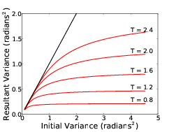 | 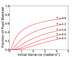 |
| (a) | (b) |
Figure 4.8: The performance of the pupil mask is defined by the balance between reducing the residual wavefront variance and minimising the fraction of the pupil being blocked. The plot on the left shows the relationship between initial variance and residual variance for a number of thresholds. The lower the threshold the greater the reduction in variance. The plot on the right shows the relationship between the initial variance and the fraction of the pupil which is blocked for a given threshold. A low threshold will result in a decreased wavefront variance but it will also require blocking a large fraction of the pupil, reducing the total intensity in the image and changing the diffraction limited PSF.
The masked phase structure function, Dϕ,APM , will have the same form as Dϕ
 but will be scaled so that it does not deteriorate as rapidly and will now converge to 2σT2. By substituting equation 4.7 into equation 4.6 the phase structure function for partially corrected wavefronts becomes,
![∫ +T 2 ∫ ∞ -8∕3
Dϕ,AO+AP M (r∕d) = 45.8 (ϕ - ¯ϕ)P (ϕ)dϕ [1- J0(ux)]H (u∕2)u du
-T 0](/wp-content/uploads/sites/167/2021/04/thesis157x.png) | (4.8) |
and for uncorrected wavefronts,
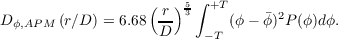 | (4.9) |
Numerical analysis of the phase structure functions indicate that they all converge towards a constant value of Dϕ(r > s) = 2σϕ2 (assuming s < L0) where s is the subaperture size in the case of partially corrected wavefronts or the diameter of the telescope for uncorrected wavefronts. From equation 2.29 it follows that the atmospheric transfer function also converges to a constant value,
 | (4.10) |
Figure 4.9 (a) shows the MTFatmos for a number of values of d∕r0, using the analytical structure functions described above. The curves can be decomposed into a Gaussian with a dc bias. The atmospheric component of the PSF will be a central peak defined by the dc offset plus a Gaussian halo with width inversely proportional to the width of the MTFatmos Gaussian component. As all the curves correspond to the same total intensity the fraction of energy within the core is given by the value of the dc offset, in this case the convergent value of the MTFatmos, and when the phase variance is low (< 1.6 radians2) the Maréchal approximation tells us that this constant is equal to the Strehl ratio. The adaptive mask will raise the convergent value (figure 2.10 (b)) increasing the fraction of energy in the diffraction limited core. Figure 4.10 shows a similar plot for the case of a telescope with no AO. In this case the MTF converges to zero. Again the pupil blocking raises this value, essentially performing the same as an adaptive optics system, flattening the wavefront and returning the ability to discern high spatial frequencies.
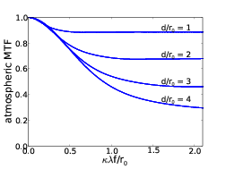 | 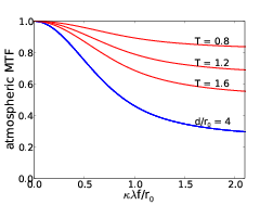 |
| (a) | (b) |
Figure 4.9: The atmospheric modulation transfer function after AO correction depends on the wavefront variance, defined by the d/r0 ratio. The left plot shows the atmospheric modulation transfer function for a range of d/r0 values as described by the analytical expression for the structure function. A lower ratio means the AO system is capable of better correction and so will converge at a higher level. Equation 4.10 states that the MTFatmos converges to exp which using the Maréchal approximation indicates the fraction of energy within the diffraction limited core. The plot on the right shows how the MTFatmos is modified by the pupil mask for a single value of d∕r0 = 4. As the threshold is reduced the system rejects more subapertures and so the residual wavefront variance is reduced, increasing the fraction of energy in the PSF core.
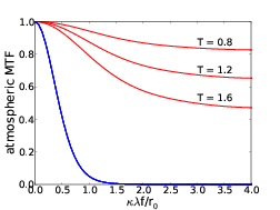
Figure 4.10: The atmospheric modulation transfer function without AO correction is shown in blue. The red lines show the MTF after pupil masking with thresholds of ± 0.8, 1.2 and 1.6 radians. Without AO or pupil masking the MTF very quickly converges to zero as the high spatial frequencies are filtered by the atmosphere.
Even if we reduce the phase variance to zero we will not be able to recover the diffraction limited PSF of the telescope. This is because we have modified the pupil function. The telescope modulation transfer function is given by the autocorrelation of the pupil function and as the adaptive pupil mask changes the shape of the telescope pupil MTFtel will also be modified. The greater the fraction of the pupil that is blocked the narrower MTFtel becomes (figure 4.11) due the lower fill factor in the pupil.
The diffraction limited point spread function, PSFdl, is given by the Fourier transform of the telescope modulation transfer function,
 | (4.11) |
The peak value in the MTF at a spatial frequency of zero corresponds to the total intensity of the PSF and the integral of the MTF will equal the peak intensity of the PSF. Therefore the narrowing of the MTF will correspond to a reduction in the peak intensity of the diffraction limited PSF. As the MTF is defined for unit intensity this will also mean a broadening of the PSF.
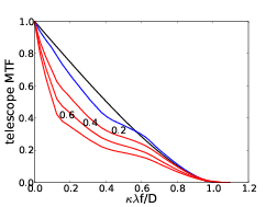
Figure 4.11: The adaptive pupil mask will have an effect on the telescope transfer function. The magnitude of this effect will depend on the fraction of the pupil that is blocked as the transfer function is given by the autocorrelation of the pupil function. The black line in the plot is the telescope MTF for a circular aperture, the blue line shows the MTF for a telescope with a central obscuration 1/4 the diameter of the primary and the red lines show the extent of modication due to the pupil mask with 20 %, 40 % and 60 % of the pupil blocked. Each plot was generated by calculating the autocorrelation function for 100 randomly blocked pupils with the required blocked fraction.
However, as we are using square blocking elements Babinet’s principle dictates that we can expect the diffraction limited PSF to be a superposition of a square diffraction pattern and the circular diffraction pattern from the pupil. The square diffraction pattern is not symmetrical and therefore examining the azimuthally averaged MTF is not enough. Figure 4.12 shows the MTFtel in two dimensions The square geometry can be seen on spatial scales corresponding to the size of the subapertures.
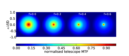
Figure 4.12: 2D telescope modulation transfer plot. The fraction of the pupil blocked by the pupil mask is 0.0 (i.e. no pupil mask), 0.2, 0.4 and 0.6. The greater fraction of the telescope pupil which is blocked the faster the MTF falls away. The central part of the MTF also becomes more square due to the square mask elements.
Figure 4.13 shows the 2D diffraction limited PSFs for increasing fractions of blocked pupil. The PSFs appear very similar except for the reduction in intensity which is proportional to the fraction of the pupil which is blocked.
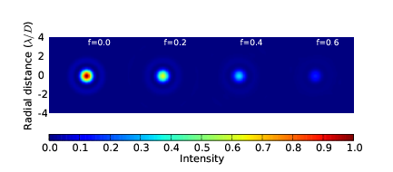
Figure 4.13: Diffraction limited long exposure PSFs for blocked pupil fractions (f) of 0.0, 0.2, 0.4 and 0.6. The secondary obstruction was one quarter the diameter of the primary. The intensity of the PSF is reduced by an amount proportional to the fraction of the pupil which is blocked. The square diffraction pattern from the pupil mask can not be seen as it is too faint.
We would expect the square symmetry in the MTF to result in a square diffraction pattern component in the diffraction limited PSF. As the mask elements are much smaller then the telescope pupil the square diffraction pattern will be larger than the primary circular diffraction pattern. Figure 4.14 shows the log10 of the diffraction limited PSFs when a fraction of 0.0 (i.e. no blocking), 0.2, 0.4 and 0.6 of the pupil is blocked. The central section of the blocked diffraction limited PSF is very similar to the non-masked PSF except reduced in intensity and reduced contrast in the minima. It is only at higher separations that the square diffraction pattern appears. In the example the pupil mask was chosen to have 8 × 8 square elements. The diffraction pattern from the mask will therefore have a minimum at approximately eight times the separation of the primary minimum of the non-masked PSF (i.e. at 8λ∕D). Greater blocking fractions will change the relative strengths between the circular diffraction pattern and the square diffraction pattern, distributing more light into the square component of the PSF. Therefore high blocking will result in a strong square diffraction pattern superimposed on the circular PSF from the telescope pupil. However, the diffraction rings are faint compared to the central core.
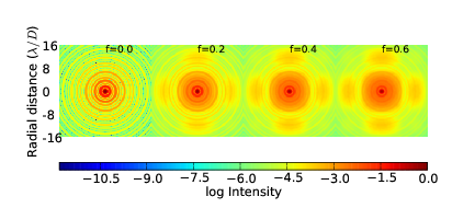 |
| (a) |
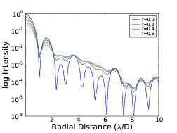 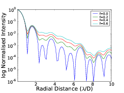 (b)(c) (b)(c) |
Figure 4.14: The colour plot shows the PSFs for the long exposure blocked apertures for blocked fractions (f) of 0.0, 0.2, 0.4 and 0.6. The secondary obstruction was one quarter the diameter of the primary. The lower plots show the radial profiles of the PSFs including the reduced intensity due to the blocking (left) and normalised to compare the structure of the PSFs (right).
The pupil mask geometry is chosen to match that of the wavefront sensor. The size of the blocking elements are fundamentally set by the number of photons entering the wavefront sensor and therefore larger telescopes will be able to support more mask elements. This will stretch the square diffraction pattern further pushing the diffraction rings away from the central part of the PSF.
The actual PSF is the Fourier transform of the product of the two modulation transfer functions (atmospheric and telescope) normalised by the fraction of the total intensity which is blocked (equation 2.25). The total MTF is shown in figure 4.15. The Fourier transform operator ensures that the area of the MTF curve is equal to the peak intensity of the PSF and the magnitude at κ = 0 is the total intensity of the PSF. We can see that the thresholds resulting in curves greater than the original will increase the peak intensity whilst reducing the total intensity, this means that the halo must be reduced.
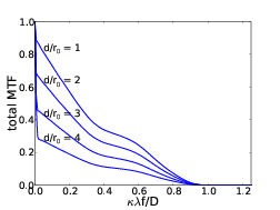 | 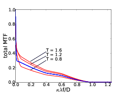 |
Figure 4.15: Combined MTF from the telescope and atmosphere, MTFatmos × MTFtel. The plot on the left shows the total MTF for AO correction with d∕r0 values of 1, 2, 3 and 4. Although it appears that the MTF curves do not all converge to 1 at κ = 0 this is not true. The telescope diameter was chosen to be 8 m and MTFatmos drops to its convergent value very quickly (~ κλf∕d (figure 2.10)) therefore MTFatmos can be considered constant. The plot on the right shows the total MTF for an 8 m telescope with 16 × 16 AO, d∕r0 = 4 and threshold values of 0.8, 1.2 and 1.6.
The simulations shown in section 4.2 (figure 4.4 and figure 4.5) assumed two test scenarios. The first was a 1 m telescope with 8 × 8 pupil masking. With a threshold of ± 1.8 radians the peak intensity was increased by a factor of 1.40 and 42% of the pupil was blocked. Figure 4.16 shows the theoretical PSF which also has a peak intensity increase of 1.4 and 40% of the pupil was blocked. We also examined a scenario with an 8 m telescope with 16 × 16 AO. The theoretical PSF again has the same peak intensity increase and the same fraction of the pupil is blocked. Therefore, the analysis agrees well with the monte carlo simulation. The actual shape of the PSFs are slightly different. This is likely to be due to additional noise sources within the the simulation (e.g. AO latency, angular geometry of the primary mirror and finite integration time).
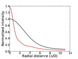 | 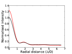 |
Figure 4.16: Theoretical PSFs for a 1 m telescope without AO and a blocking threshold of ±1.8 radians (left) and an 8 m telescope with AO and a threshold of ±1.4 radians (right). The peak intensity increase and the fraction of the pupil which is blocked agrees well with the PSFs generated by the monte carlo simulation (section 4.2, figure 4.4 and figure 4.5).
We can now calculate the expected PSF from the input parameters (immediate seeing, telescope pupil function and number of subapertures) and calculate the optimum threshold for maximum peak intensity. Given extra parameters for a binary system (magnitude difference and separation) the optimum threshold for faint companion detection can also be calculated. This will be a combination of increased peak intensity and reduced PSF halo which do not necessarily correspond to the same threshold. It might even be beneficial to run a very low threshold to reduce the phase variance significantly and use PSF subtraction techniques to remove the square diffraction pattern, as this will allow for a much reduced halo.
4.4 High contrast imaging
Modern extreme AO systems are capable of reducing the atmospheric seeing to near diffraction limited over a small field of view and any residual wavefront error after the AO system are random and will average out over time. The direct imaging of extrasolar planets is now limited by static speckles. Speckles caused by misalignment of optics and aberrations in the mirrors. These speckles will not average and may cause false positives, i.e. be erroneously identified as planets. They can not be subtracted either as although appearing static they do actually vary with time as the telescope moves and the temperature changes.
There are now many static speckle removal techniques. Ribak & Gladysz [76] suggest that the speckles can be removed by breaking the symmetry in the optical system. By apodizing the primary with a rotating off-axis circular mask the speckles will now move in the focal plane and average out. However, the position of the star and planet will remain fixed. The adaptive pupil mask could also be used in a similar way to break the symmetry as different areas of the pupil are blocked.
The diffraction pattern due to the mask will be chromatic. Although this might be a problem for imaging white light it is also possible that it could be used in some way to further reduce the speckles. It is also possible that the technique might be useful for larger telescope D > 8 m in order to help reduce residual wavefront error, although that is a discussion for future work.
4.5 Conclusions
We have presented a novel technique for improving the quality of a PSF in terms of increasing peak intensity and reducing the halo. Light from areas of a telescope pupil which are out of phase will not add to the core but instead create a diffuse halo. By blocking the appropriate subapertures we obtain a much flatter wavefront and by controlling the extent of the blocking we can maximise the peak intensity and minimise the PSF halo. If we block too much the diffraction limited PSF becomes broader and the peak intensity will be compromised. If we do not block enough there will be subapertures with large piston error remaining. The performance of the adaptive pupil mask is most dramatic in systems with a large fraction of energy in the halo but can also provide significant improvements for higher Strehl images.
The optimum threshold is a function of initial phase variance and the ratio of subaperture size to telescope diameter. A theoretical explanation of the pupil mask has been developed in order to estimate the optimum phase threshold as a function of initial phase variance. The two examples shown in this chapter are for two different scenarios but the technique will work in any instance where the wavefront is properly sampled.
In simulations the peak intensity for a 1 m class telescope can be increased by 40 % and the FWHM reduced by 76 % to near the diffraction limit. This was done by blocking any subaperture with a piston excursion greater than 1.8 radians. For an 8 m class telescope equipped with AO the adaptive pupil mask can increase the peak intensity by 23 % and the FWHM reduced from 0.022 ” to 0.018 ”. The reduced FWHM and increased peak intensity is beneficial for the direct imaging of faint companions as the contrast ratio will be reduced.
Simulations show that the SNR for a 100 s exposure observing a faint companion at an angular separation of 2λ∕D from the primary star with a magnitude difference of 7.7 on a 1 m telescope is 5. The inclusion of the adaptive pupil mask double this to 10.5. A binary system of the same separation but magnitude difference of 11.7 on an 8 m telescope also has a SNR of 5. The addition of a four-quadrant phase mask coronagraph results in an increase to 6.6 which is comparable to the addition of the pupil mask. If the pupil mask is used before the coronagraph a SNR of 10.6 is achieved due to the reduced FWHM resulting in a more efficient coronagraph.
It is perhaps unlikely that this technique will be of use to modern planet imaging projects which use very high order AO systems (extreme AO) and are now limited by static speckle rather than residual phase. However, it could be useful for smaller telescopes as a relatively easy way to increase the imaging resolution.
Digital Micromirror Device [77] technology is now reaching a very developed stage and could easily handle the update rates and chip sizes required of the adaptive pupil mask and could be used in the pupil plane of the telescope to reflect the appropriate sections of the wavefront out of the optical path. For a telescope with no AO capabilities the pupil mask could be implemented with a beam splitter, a Shack-Hartmann wavefront sensor and a DMD. A telescope already equipped with an AO system can share the wavefront sensor and so only requires positioning the DMD in the optical path after the deformable mirror.
Chapter 5
Scintillation Reduction
5.1 Introduction
5.2 Opto–mechanical design
5.3 Scintillation Calibration
5.4 Theory and Simulation Results
5.5 Performance Estimation
5.6 Conclusions
5.1 Introduction
High precision fast photometry from ground based observatories is a challenge due to intensity fluctuations induced by the Earth’s atmosphere. Here we describe a method to reduce this noise source by conjugating the pupil to the altitude of a high dominant turbulent layer. We reduce the scintillation from this layer by apodising the pupil and normalise with a comparison star to remove the scintillation we now obtain from the lower layers. We find by simulation that given a simple atmosphere with a single high altitude turbulent layer and a strong surface layer a reduction in the intensity variance by a factor of ~30 is possible. Given a more realistic atmosphere as measured by SCIDAR at San Pedro M rtir we find that on a night with a strong high altitude layer we can expect the median variance to be reduced by a factor of 7.8. By reducing the scintillation noise we will be able to detect much smaller changes in brightness. If we assume a 2 m telescope and an exposure time of 30 seconds a reduction from 0.76 mmag to 0.26 mmag is possible, which will enable the routine detection of, for example, the secondary transits of extrasolar planets from the ground. If ultimately successful, the techniques developed here would usher in a revolution with very-high precision photometric instruments, deployable on easily accessible 1 to 2 meter class telescopes, which would be capable of detecting highly-prized bright Earth-like exoplanets and characterizing the atmospheres of known transiting exoplanets. This capability would make this relatively low-cost instrument competitive with the science goals of much larger planed projects, such as the dedicated space mission of PLATO[5].
5.2 Opto–mechanical design
The design of a conjugate-plane photometry is actually very simple. Figure 5.1 is a diagram of such an instrument. An aperture is placed in the collimated beam at the conjugate plane of the turbulent layer. A lens is then used to focus the light onto a CCD in the focal plane. As the aperture is not in the pupil plane, any off-axis light will not illuminate the whole aperture and therefore a separate optical arm is required for the target and comparison star. This can be achieved with either a prism near to the focal point of the telescope, or with pick off arms if more stars are required. This is completely different to an adaptive optics type approach as there are no moving parts once the altitude has been set.
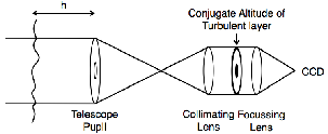
Figure 5.1: Conceptual design for one arm of the instrument.
Figure 5.2 shows the full design of a prototype instrument which shall shortly be commissioning to demonstrate the conjugate-plane photometry technique. The optics were designed by Richard Wilson and mechanical design by Simon Blake and the author was responsible for all of the simulations and data reduction.
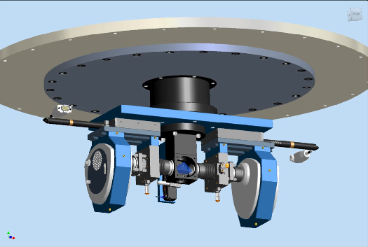
Figure 5.2: Prototype of the conjugate-plane photometer, that we are due to test on-sky shortly.
5.3 Scintillation Calibration
High altitude turbulence in the atmosphere distorts the plane wavefronts of light from a star which is effectively at infinity. As the wavefronts propagate these phase aberrations evolve into intensity variations which we view with the naked eye as twinkling. Wavefronts incident on a telescope pupil have both phase variations, caused by the integrated effect of light passing though the whole vertical depth of the atmosphere, and intensity variations, caused predominantly by the light diffracting through high altitude turbulence and interfering at the ground. Phase variations are normally considered more significant as they dramatically affect the spatial resolution of the images, and this has led to the development of adaptive optics. The intensity variations across the pupil are effectively averaged together when the light is focused and therefore have less effect. A larger aperture implies more spatial averaging (which is why stars twinkle less when observed through a telescope than with the naked eye). However, these small intensity fluctuations do become significant when one is concerned with high precision photometry.
Consider now the effect of these intensity variations in more detail. If we ignore diffraction, then a flat wavefront which is the same size as the telescope pupil at a given high altitude, in the absence of atmospheric turbulence, will propagate in a direction normal to the wavefront and will be collected by the telescope pupil (see figure 5.3). Now consider the effect of atmospheric distortion. Phase aberrations cause diffraction in different directions and hence produce scintillation. Effectively light from one part of the original wavefront is redirected to other parts of the pupil. This in itself is not a significant problem for photometry, as the integrated intensity across the pupil is the same. The problem occurs either when rays from the wavefront at high altitude propagate away from the telescope pupil, and are lost, or conversely when high altitude areas away from the telescope pupil area propagate into the telescope pupil at the ground. These effects lead to a decrease and increase in intensity, respectively, and at any one instant both of these effects will be occurring (see figure 5.3).The turbulence is blown across the field of view of the telescope producing an overall change in intensity as a function of time.
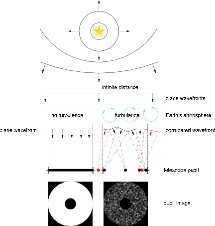
Figure 5.3: A spherical wavefront from a star will appear flat as it enters the the atmosphere. In the absence of turbulence this flat wavefront will be collected by the telescope pupil (left). In the presence of turbulence the wavefront will diffract through the refractive index variations which accompany the turbulent motion in the atmosphere. The wavefront will then interfere with itself at the ground and cause intensity fluctuations. A simplified geometrical model is shown on the right. The scintillation noise occurs when extra light is focused into the telescope pupil or when light is focused away from the pupil by the turbulent atmosphere. (Diagram courtesy of V. Dhillon)
As a thought experiment, to show the basic concept behind our proposal, if we could place an aperture which is smaller than the telescope pupil in the sky at the altitude of high turbulence then this change in intensity could be dramatically reduced. In this case, the rays that would have been deflected away from the area of the pupil would still be collected by the (larger) telescope pupil, and as the angle of diffraction is small no rays would be deflected into the telescope pupil because of the aperture (figure 5.4). Increasing the size difference between the aperture in the sky and the telescope pupil would improve the scintillation rejection, but would also lead to increased loss of signal, and clearly a balance between the two effects would need to be found.
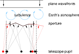
Figure 5.4: By placing an aperture at the altitude of the turbulent layer we can reduce the scintillation noise. It will now be impossible for any light from outside of the telescope pupil to be focused into the collecting area. It will also be unlikely for any parts of the wavefront to be focused off-axis by such a degree as to escape from the collecting area all together. These two situations are shown in red. These rays – which would normally be the ones producing a change in the overall intergrated intensity – are blocked. (Diagram courtesy of V. Dhillon)
Clearly placing an aperture at a high altitude in the sky is an impractical proposal, but we can produce a similar effect using optics after the telescope focus. Figure 5.5 shows how reconjugation can be produced by observing the beam in a different plane downstream from the telescope focus. The high altitude turbulent layer is reimaged onto an aperture which is slightly smaller than the equivalent size of the full telescope pupil. Consider again the simplified case of a single layer of turbulence at a high altitude. As already described, this produces scintillation in the entrance pupil of the telescope. If we reimage the high altitude layer at a conjugate plane then the rays will have propagated so as to “undo” the scintillation and we would view an approximately uniform intensity [78]. High altitude areas of the wavefront, which in the absence of turbulence would fall outside of the telescope pupil, can be diffracted by the turbulence and interfere to cause intense regions within the pupil area. This light would image in the conjugate plane outside of the aperture and can be easily rejected by the mask. High altitude areas of the wavefront which are diffracted by the turbulence and interfere to cause intense areas at the ground outside of the telescope pupil are lost and will show up as areas of decreased intensity towards the edge of the reimaged wavefront. This effect can also be rejected with a mask at the reimaged altitude which is slightly smaller than the pupil size. The remaining light within this mask will be approximately of uniform intensity and scintillation free.
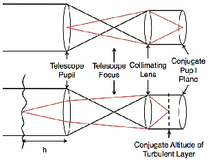
Figure 5.5: Ray diagrams for conjugation positions. The black lines show the rays for an object at infinity. The top diagram shows the conjugate position of the telescope pupil. Every point in this plane will be an image of a point on the telescope pupil (as shown by the red lines). The lower diagram shows that by moving the observation plane towards the collimating lens then an image of the wavefront at a height h above the telescope will be produced. If a camera is in a position such that it is in the image plane of the turbulent layer it is at the conjugate altitude of that layer. In practice subsidiary optics may also be used, but this diagram shows the principle.
The above description has ignored two important effects, namely diffraction and turbulence from other atmospheric layers (predominantly low altitude turbulence). In the far field the intensity pattern will have developed into the well known Airy diffraction pattern and so will not change shape with propagation distance. In the near field the diffraction pattern will develop with distance which makes it more complicated to calculate. The Fresnel number, F, is used to determine which set of approximations are valid and is given by,
 | (5.1) |
where Dtel is the diameter of the telescope pupil, z is the propagation distance and λ is the wavelength of the light. For F ≪ 1 far field Fraunhofer diffraction can be assumed, if F > 1 we are in the near field and so Fresnel diffraction theory is valid. In all astronomical cases the apertures are large enough that Fresnel diffraction is always valid at optical wavelengths.
Figure 5.6 shows simulated images of reconjugated pupils for telescopes with diameters, D = 0.4, 1.0, 2.0, 4.0 and 8.0 m and for reconjugated altitudes 0 m (telescope pupil), 1000 m, 5000 m and 10000 m. At higher altitudes we see ringing in the pupil. This ringing is caused by diffraction of the wavefront through the telescope pupil and so larger telescope pupils or shorter propagation distances result in less diffraction and less ringing. The Fresnel number is also shown underneath each plot. The diffraction rings are not constrained to the outer edge of the pupil they actually permeate through the entire pupil with exponentially decreasing amplitude as described by the Fresnel diffraction integral.
| z = 0 m | z = 1000 m | z = 5000 m | z = 10000 m | |
| D = 0.4 m |  | 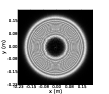 | 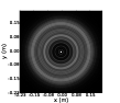 | 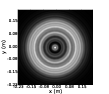 |
| (F = ∞) | (F = 80) | (F = 16) | (F = 8) | |
| D = 1.0 m | 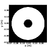 |  | 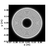 | 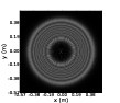 |
| (F = ∞) | (F = 500) | (F = 100) | (F = 50) | |
| D = 2.0 m | 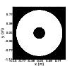 | 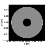 | 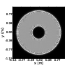 | 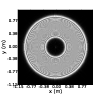 |
| (F = ∞) | (F = 2000) | (F = 400) | (F = 200) | |
| D = 4.0 m | 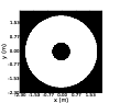 | 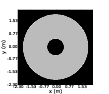 | 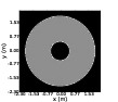 |  |
| (F = ∞) | (F = 8000) | (F = 1600) | (F = 800) | |
| D = 8.0 m |  | 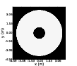 | 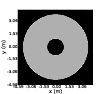 |  |
| (F = ∞) | (F = 32000) | (F = 6400) | (F = 3200) |
Figure 5.6: Re-conjugated pupil intensity images for a number of aperture diameters and increasing propagation distance. The Fresnel number is also shown as an indication of the amount of diffraction. F ≪ 1 indicates far field (Fraunhofer) diffraction. The images do not include any turbulence, only diffraction.
In addition to high altitude turbulence most astronomical sites will also have a strong surface layer [11, 13] and possibly turbulence at intermediate altitudes as well. If we conjugate our system to the altitude of a high turbulent layer we will still see scintillation from other layers. We will have effectively swapped scintillation caused by high altitude turbulence with scintillation caused by turbulence close to the ground. Fuchs et al. [78] demonstrated that if a turbulent layer is below the conjugate plane (the surface layer for example) then a virtual reverse propagation occurs over a distance z = |h – z0|, where z0 is the conjugate altitude and h is the altitude of the turbulent layer. Therefore the surface layer will now cause scintillation in the conjugate plane as it will have effectively propagated a distance z0. However a comparison star can be used to reduce the scintillation from the surface layer as they will both sample the same turbulent area, as shown in figure 5.7. This layer must also be quite thin to ensure the wavefronts sample the same turbulence, and studies have demonstrated that this is the case (it is often only a few 10’s of meters, [11, 13, 50]) meaning that the isophotometric angle is now very large (up to 0.5∘).
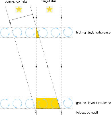
Figure 5.7: In differential photometry the intensity of the target star is calibrated by the intensity from a second comparison star. As the scintillation is caused by high altitude turbulence the two light cones do not sample the same turbulence and hence there will be very little correlation between the two. By conjugating the telescope to the high-altitude layer we remove the scintillation from this layer and it is replaced by scintillation from the surface turbulent layer instead. However, as the two light cones sample the same region of turbulence near the ground they will have very similar scintillation patterns, allowing one to be corrected by the other. The angle of separation of the two stars can be large as the surface layer is generally found to be thin. (Diagram courtesy of V. Dhillon)
Figure 5.8 shows the effect of reconjugation of a single high altitude layer, including the effects of diffraction caused by the telescope pupil. The simulation assumed a single high altitude turbulent layer at 10 km with ∫ Cn2dh = 353 × 10-15 m1∕3, where Cn2 is the refractive index structure constant and ∫ Cn2dh is the integrated turbulence strength of the atmospheric layer. This corresponds to r0 = 0.15 m, where r0 is the Fried parameter and is a measure of the integrated strength of the turbulence. It can be seen that the variations in intensity due to scintillation largely disappear in the reconjugated image of the high altitude layer – but that diffraction can clearly be seen. The diffraction rings are not completely circular as a result of the phase distortions in the wavefront at the telescope pupil. Figure 5.9 shows simulated images of the reconjugated pupils at 10 km for a two-layer atmosphere (0 and 10 km) for two stars separated by 40′′. The two images are very similar indicating that one may be used to calibrate the other. They are not identical, however, due to the high altitude turbulence (and not the finite thickness of the layer) illuminating the surface layer with an aberrated wavefront. As this initial aberration is different for the two stars the intensity distribution in the conjugate plane will also be different, and this introduces a source of error – as described in more detail in the next section.
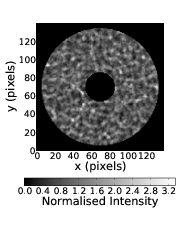 | 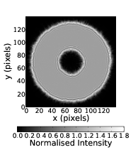 |
Figure 5.8: Simulated pupil intensity patterns at the telescope pupil (left) and at the conjugate altitude of the turbulent layer (right). The telescope pupil is 2.0 m in diameter and the turbulent layer has ∫ Cn2dh = 353 × 10-15 m1∕3 and is located at an altitude of 10 km. The intensity pattern at the conjugate altitude shows that the spatial intensity fluctuations have been removed but have been replaced by diffraction rings concentrated around the edges that also permeate throughout the pupil.
 |  |
Figure 5.9: Pupil images conjugate to 10 km for two stars separated by 40′′. The spatial intensity fluctuations are a combination of the scintillation pattern from the surface turbulent layer and the diffraction pattern of the telescope pupil (figure 5.8, right). The two images have very similar intensity patterns as they are both formed by the propagation of the same area of surface layer.
5.4 Theory and Simulation Results
Assuming a single turbulent layer at 10 km and no other turbulence the wavefunction, Ψ, at the telescope pupil is given by,
![Ψ(x,y) = [K(z = +10 km)⊗ exp(iϕ10)]P (x,y),](/wp-content/uploads/sites/167/2021/04/thesis207x.png) | (5.2) |
where z is the propagation distance, x and y are spatial co-ordinates, P(x,y) is the telescope pupil function, ϕh is the turbulent phase screen at altitude h km, ⊗ denotes a convolution and K is the Fresnel propagation kernel, given by,
![( [ ])
K = i-exp(ikz)exp ik (x- x′)2 + (y- y′)2 ,
λz 2z](/wp-content/uploads/sites/167/2021/04/thesis208x.png) | (5.3) |
where k is the wavenumber λ is the wavelength of the light and x′ and y′ and spatial co-ordinates in the observation plane located at a distance z. Positive z indicates a diverging spherical wavefront and negative z is a converging spherical wavefront or a negative propagation. Therefore, the wavefunction in the conjugate plane, Ψ′(x′,y′), is found by a further propagation of the wavefront by a negative distance,
![Ψ′(x ′,y′) =
K (z = - 10 km )⊗ [[K(z = +10 km)⊗ exp (iϕ10)]P (x,y)].](/wp-content/uploads/sites/167/2021/04/thesis209x.png) | (5.4) |
In the case of an infinitely large pupil, Ψ′(x′,y′) = Ψ(x,y) and the pupil amplitude is flat. Therefore, by placing the aperture at the conjugate altitude of the turbulent layer we can reduce the scintillation caused by that layer. However, with a real aperture the intensity profile at the conjugation plane is not flat because the wavefront diffracts through the telescope pupil and causes diffraction rings at the edge of the pupil image which are a function of the turbulent phase screen. If we include a ground layer, ϕ0, the Fresnel propagation equation becomes,
![′ ′ ′
Ψ (x ,y) = K(z = - 10 km)
⊗ [[K (z = +10 km )⊗ exp(iϕ10)]exp(iϕ0)P (x,y)].](/wp-content/uploads/sites/167/2021/04/thesis210x.png) | (5.5) |
The surface layer and telescope pupil are multiplied into the wavefront before the final convolution. This is why these effects can not be de-coupled from the higher turbulent layers and the wavefront in the conjugate plane will therefore depend on the high altitude phase aberrations as well as the surface layer and will be different for the target and comparison stars. In addition to the diffraction these residual intensity variations will limit the effectiveness of the technique.
Our conjugate-plane photometry concept has been simulated using a modification to the simulation described in section 2.5.2. The simulation is a Fresnel propagation wave optics simulation using the theory stated above and randomly generated phase screens. It has been modified to propagate two beams through each phase screen at the appropriate displacement depending on the layer altitude. The simulation has also been modified to back propagate the wavefronts to the conjugate plane where they are masked and sampled.
Scintillation is often quantified by the scintillation index, σscint2, which is defined as the normalised variance of intensity fluctuations, σscint2 = ⟨(I -⟨I⟩)2⟩∕⟨I⟩2, where I is the intensity of the image and ⟨I⟩ denotes the time averaged intensity [39]. Figure 5.10 shows the scintillation index as a function of aperture size for a few example cases. The first case shows the theoretical maximum reduction found by suspending the aperture in the sky above the telescope (solid line). This is entirely unfeasible but places a maximum limit on the reduction of the variance. The black dot–dashed line shows the scintillation variance for differential photometry with the aperture in the conjugate plane. Diffraction through the pupil means that light is redistributed in the pupil and will result in a higher scintillation variance. The small shoulder in the curve at approximately 0.07 m coincides with the radius of the first diffraction ring. The red dashed lines show the scintillation variance with a high altitude layer and a surface layer which varies in strength. In this case a comparison star is required to normalise the scintillation. The strength of the surface layer is selected so that the ratio of Cn2(10 km)dh∕Cn2(0 m)dh is equal to 1, 2 and 4. If the surface layer is weaker than the high turbulent layer the residual intensity fluctuations will be lower. The maximum median variance reduction factor for Cn2(10 km)dh∕Cn2(0 km)dh = 1 (i.e. equal strength), 2 and 4 is 17, 23 and 47, respectively and is found at Daperture – Dtel ≈ 0.1 m, for a simulated telescope diameter of 2 m.
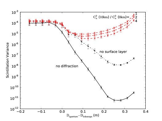
Figure 5.10: The solid line shows the scintillation variance as a function of aperture size for an aperture suspended in the sky 10 km above a 2 m telescope. In this case it is possible to reduce the scintillation variance to effectively zero. The black dot–dashed line shows the scintillation variance for a single high-altitude turbulent layer with the aperture in the conjugate plane. The performance is not as good as the solid line due to the diffraction from the telescope pupil. The red dashed lines show the scintillation variance for the aperture in the conjugate plane of the high turbulent layer and with a surface layer with strengths equal to Cn2(z0)dh, 2 ×Cn2(z0)dh and 4 ×Cn2(z0)dh, where z0 is the conjugate altitude, with Cn2(z0)dh = 3.5 × 10⁻¹³m1∕3. For small apertures there is less averaging of the intensity fluctuations resulting in increased scintillation index. Due to the aperture dependance of scintillation index, when using very small apertures we expect the index to increase as shown in the figure. The data points and error bars are the mean and standard errors of 20 simulations, each with unique and randomly generated phase screens.
The amplitude of the first diffraction ring is substantially larger than any others (as seen in figure 5.8). The optimum aperture size is therefore one which blocks this ring but none of the others. This will minimise the residual diffraction and retain a large pupil area. The radius of the first diffraction ring in the very near field is given by the radius of the first Fresnel zone, rF =  , in this case 0.07 m (the location of the shoulder in the figure) and is independent of telescope size.
Figure 5.11 shows the four possible light curves, the two normal light curves, one from each target star, in the focal plane and the two reconjugated and masked light curves. The normal light curves for the two target stars have no correlation as the scintillation is caused by the high altitude turbulence. However, the reconjugated pupils are well correlated as the variations are caused by the surface layer which is common to both stars and so can now be removed.
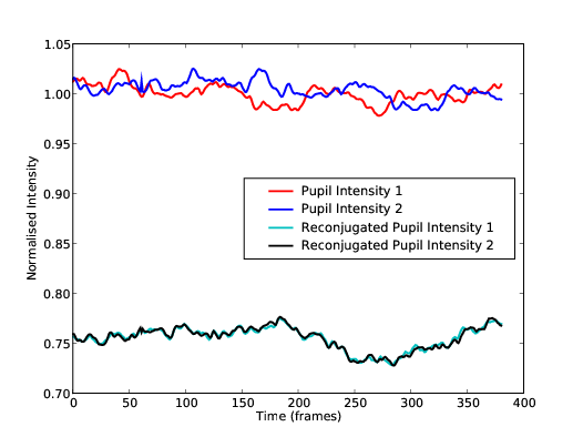
Figure 5.11: Example simulated light curves for the normal and reconjugated pupils. The red and blue lines are the light curves for each target star. The variations are caused by the high altitude turbulence and so are uncorrelated. The black and turquoise light curves are simulated after the conjugate-plane photometer and are well correlated as the variations are now caused by the low altitude turbulence which they both sample. The simulation assumed a 2 m class telescope observing through an atmosphere with a turbulent layer at 10 km and 0 m, both with ∫ Cn2dh = 353 × 10-15 m1∕3. The exposure time of each frame is short so that there is no temporal averaging of scintillation.
The reduction in scintillation noise can be clearly seen in figure 5.12, which shows the normalised light curve for a sequence of 385 frames from a simulation assuming a constant source intensity. The black line shows the original light curve with a variance of 1.5 × 10⁻⁴, due to scintillation. The red line is the light curve after scintillation reduction and has a variance of 6.1 × 10⁻⁶, a reduction factor of 20. The variance is in units of normalised intensity, ΔI∕I. The simulation assumes an atmosphere with two turbulent layers, one at the ground and one at 10 km, both with ∫ Cn2dh = 353 × 10-15 m1∕3 (r0 = 1.15 m), the telescope diameter was 2 m and there was no temporal averaging.
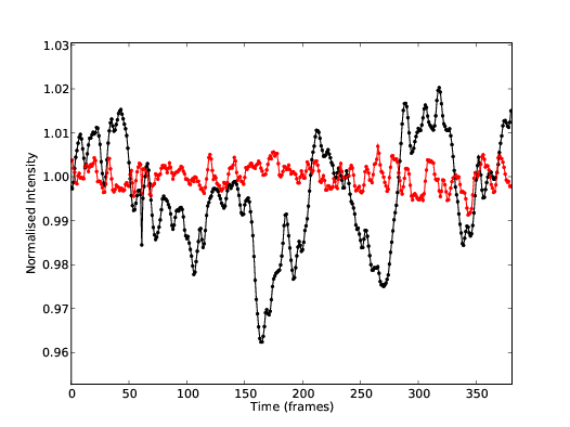
Figure 5.12: An example simulated light curve. The black line is the intensity pattern from a simulation observing a star with a 2 m class telescope through the atmosphere with a turbulent layer at 10 km and 0 m, both with ∫ Cn2dh = 353 × 10-15 m1∕3. The exposure time of each frame is short so that there is no temporal averaging of scintillation. The red line shows the scintillation corrected light curve. In this case the intensity variance is reduced from 1.5×10⁻⁴ to 6.1×10⁻⁶, a factor of 20. The residual noise is due to the uncorrected scintillation.
A mis-conjugation of the aperture will result in less than optimal performance. Figure 5.13 shows the factor by which the scintillation variance is reduced as a function of conjugate altitude for a turbulent layers at 0 m and a layer at 6, 8, and 10 km. In the 10 km case the curve has a full width at half maximum of approximately 3.5 km. This will be higher and narrower for turbulent layers at lower altitudes and lower and wider for higher altitudes. The maximum correction reduces at higher altitudes due to the extra propagation distance meaning that the scintillation is stronger. The curve also broadens at higher altitude as the residual scintillation due to mis-conjugation is small compared to the scintillation due to the propagation from the turbulent layer to the ground. Knowledge of the contemporaneous turbulence profile is therefore essential to ensure that the aperture is conjugate to the correct altitude.
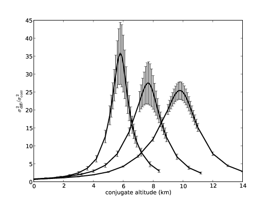
Figure 5.13: Ratio of intensity variance for normal differential photometry (σdiff2) and scintillation corrected photometry (σcorr2) versus conjugate altitude for an atmosphere with a layer at 0 m and a layer at 6, 8, and 10 km, all with ∫ Cn2dh = 353 × 10-15 m1∕3 and a telescope diameter of 2 m. The curves are Lorentzian and the 10 km curve has a FWHM of approximately 3.5 km. At conjugate altitude 0 m we measure an improvement in the intensity variance of ~0.5, i.e. the variance is actually increased. This is because the pupil size is reduced by the apodizing mask. The data points and error bars are the mean and standard deviation of 20 simulations, each with unique and randomly generated phase screens.
In the examples so far we have only considered profiles with two layers (a high turbulent layer and the boundary layer). However, if a third layer is present we will obtain scintillation from this layer at the conjugate altitude. If this third layer is high so that it is not common to both stars it can not be cancelled out in the same way as the ground layer. Figure 5.14 shows the scintillation calibration technique response to a third layer at an altitude (h3). In the simulation we assumed the third layer was the same strength as the other two layers i.e. r0 = 0.15 m. It is found that when the third layer is near to the altitude of the second layer the improvement factor is high and when the distance between the two layers is increased the improvement factor reduces as expected.
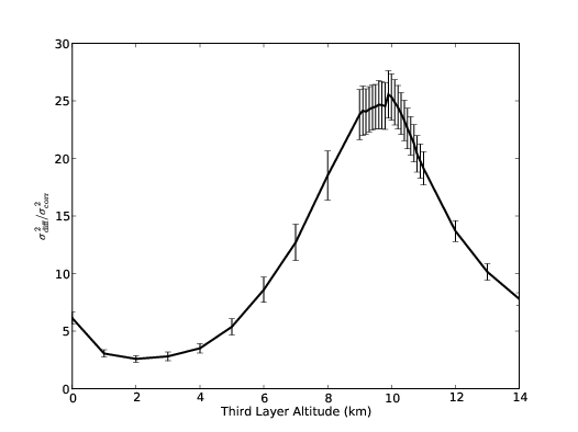
Figure 5.14: Instrument sensitivity to additional turbulent layers at intermediate altitudes. The fixed two layers are set at 0 m and 10 km and all the layers have an r0 = 0.15 m. The position of the minimum is determined by the separation of the target stars. When the third layer is located close to the ground it can be partially removed by normalisation. Therefore, the minimum will occur when the two light cones are separated by one coherence length and can not be normalised.
5.5 Performance Estimation
The Monte-Carlo simulations are useful to examine the performance for a particular parameter set. However, it is very inefficient for modelling the performance as a function of time for real turbulence profiles with many turbulent layers. To do this an analytical estimate of the intensity variance for a given parameter set is required.
If the pupil is much larger than the Fresnel radius (D ≫ ) the intensity variance due to scintillation, σscint2, can be predicted using the theoretical model described by Dravins et al. [40],
 | (5.6) |
where γ is the zenith angle. The scintillation index is then independent of wavelength and proportional to the altitude of the turbulent layer squared and the strength of the turbulent layer. We can calculate the scintillation index due to all of the turbulent layers assuming the pupil is conjugate to an altitude, z0. In this case the scintillation index, σz02, at a given altitude can be calculated using a modification to the scintillation index equation (equation 5.6),
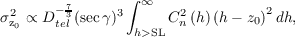
where (h – z0) is the separation between the layer altitude and the conjugate altitude, ignoring the surface layer as this will be dealt with separately.
The corrected residual scintillation variance, σcorr2, will be dominated by this but we also add noise terms due to the pupil diffraction and the surface layer. These noise sources are independent but the total is modulated by the original scintillation variance (equation 5.5) and so the total residual scintillation variance can be modelled by,
 | (5.8) |
where σSL2 is the scintillation index due to the surface layer, F is the Fresnel number used to quantify the ‘amount’ of diffraction and is given by F = Dtel2∕4λz, and j, k and l are solved empirically from the simulation results and are found to be j = k = 0.66 ± 0.09, l = -1.4 ± 0.05. In this case it is important to note that the σz02 and σSL2 should both be calculated with the diameter equal to the size of the aperture and not the telescope pupil.
Figure 5.15 shows a comparison between the simulated data and the predicted values from equation 5.8. Each curve represents the scintillation variance as a function of conjugation altitude for a layer at the ground and 6, 8, 10 or 12 km. The parameters were also tested and for telescopes of varying sizes and layers of varying strengths.
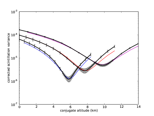
Figure 5.15: Comparison of simulated and predicted corrected scintillation variance for turbulent layers at 0 m (all curves) and 6, 8 and 10 km, the telescope diameter is 2 m and there was also a turbulent layer at the ground of equal strength as the higher layer. The solid black lines with error bars are the mean of 20 unique simulations, the error bars indicated the standard error on the value. The coloured lines are the predicted values using equation 5.8. The reduced χ2 value is 1.9.
Using high-resolution generalized SCIDAR turbulence profile data from San Pedro M rtir [79] and the model developed from the simulation results we can estimate the expected improvement in intensity variance. The SCIDAR profile shown in figure 5.16 was recorded on 19th May 2000 and shows a strong turbulent layer at approximately 10 km throughout the night. Figure 5.17 shows the expected improvement factor in intensity variance as a function of time for the same night. The median improvement ratio is 11.5 for this example.
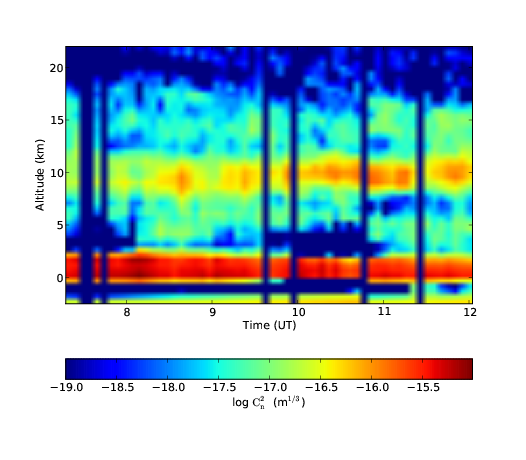
Figure 5.16: SCIDAR turbulence profile, i.e. the height above sea level against time, where the colour indicates the strength of the turbulence, from 19th May 2000 at San Pedro M rtir. The profile shows a dominant layer at approximately 10 km throughout the night. San Pedro M
 rtir is located at 2800 m above sea level.
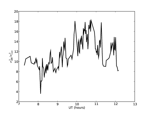
Figure 5.17: Predicted improvement in intensity variance as a function of time for the night of 19th May 2000. The median improvement ratio for this night is ~11.5.
Figure 5.18 shows the actual scintillation variance and the scintillation corrected variance expected on the 19th May 2000.
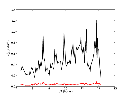
Figure 5.18: Predicted scintillation variance as a function of time for the night of 19th May 2000. The black line is the expected scintillation variance for differential photometry and the red line is the scintillation corrected variance.
When calculating expected performance for real experiments it is also necessary to include the exposure time of the integration as this will average out the scintillation and reduce the intensity variance. The scintillation index given in equation 5.6 is only valid for very short exposures where there is no temporal averaging, i.e. the exposure time has to be less than the pupil crossing time of the intensity fluctuations. The crossing time, tc, can be calculated as tc = Dtel∕vw, where vw is the velocity of the turbulent layer. If the exposure time, t, is greater than the crossing time then the scintillation index is modified to [43],
 | (5.9) |
where V (h) is the velocity of the turbulent layer at altitude h. Using this modification to the scintillation index we can calculate an example light curve for a fictional extrasolar planet transit for a given turbulence profile.
Figure 5.19 shows an example simulated extrasolar planet transit. The transit depth is assumed to be 0.05 %, i.e. it is of a depth typical for the secondary transit when the planet passes behind the star, and has a duration of 2.5 hours. A 2 m telescope and 30 s exposure time are also assumed. The optical turbulence profile used in the simulation is the same as that shown in figure 5.16 as measured by SCIDAR at San Pedro M rtir. A wind speed of 5 ms-1 for the surface layer and 20 ms-1 for all other turbulence is assumed. The normalised scintillation noise in the visible is reduced from 0.70 × 10⁻³ (0.78 mmag) to 0.21 × 10⁻³ (0.23 mmag), an improvement factor of 3.3 (10.9 in variance). If we assume a target magnitude of 11 then we have reduced the scintillation to a level which is comparable to the shot noise.
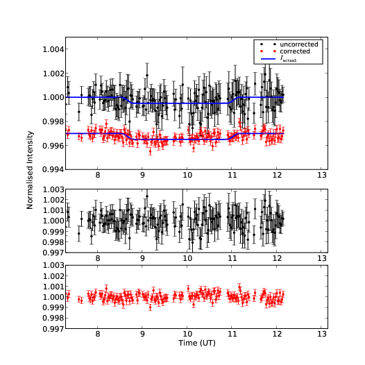
Figure 5.19: Simulated light curve of a secondary transit of an extrasolar planet with a 0.05% transit depth. The data were calculated assuming the same atmospheric parameters as measure by SCIDAR (figure 5.16) and a 2.0 m telescope with 30 s exposure times in the v-band and a target magnitude of 11. The top panel show the simulated light curves with no scintillation correction (black points, top) and with scintillation correction (red points, bottom), offset for clarity. The blue lines show the theoretical light curve (i.e. with no noise). The data points are randomly selected from a distribution with a variance equal to the total noise at that time, and the error bar indicates the total noise at that time. The lower panels show the normalised residuals.
Although the aperture must be placed at the conjugate altitude of the turbulence the photometry can be done in the focal plane. This means that we do not expect any of the other noise sources to increase as a result of implementing our conjugate-plane photometry technique. However, as the scintillation is now caused by the lower turbulent layers which will inherently have a lower wind speed the photometry fluctuations will take longer to average out. The magnitudes of other noise sources such as shot noise, readout noise or flat fielding noise will depend on other factors. There are three possible regimes in which we are interested: scintillation dominated, other noise dominated and a mixture of the two. In the first and last cases the noise will add in quadrature and so a reduction in scintillation noise by a factor of n will reduce the total noise to, σT2 = , where σT is the total noise before scintillation reduction. Figure 5.20 shows a 2D plot of the total noise reduction factor as a function of the telescope diameter and the target magnitude assuming the same parameters as before. The atmospheric model was the median profile from the SCIDAR data recorded on 19th May 2000. The optimum telescope size is found to be between 1.2 m and 2 m. Less than this and the diffraction effects limit the possible scintillation noise reduction and apertures greater than this become shot noise dominated. In the latter scenario the scintillation noise is insignificant and so scintillation correction techniques will have no effect.
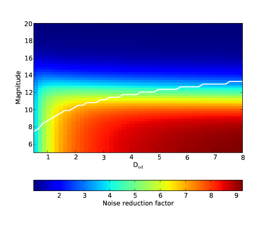
Figure 5.20: The magnitude of the improvement we can expect to observe with conjugate-plane photometry depends on the other noise sources. If we assume the same parameters as in figure 5.19 and an atmosphere given by the median SCIDAR profile then we can plot the noise reduction factor as a function of target magnitude and telescope diameter. The white line indicates the limiting magnitude for a given telescope size to prevent saturating a 16 bit analogue to digital converter in a CCD. The optimum telescope size is therefore the maximum reduction factor just above this curve, i.e. between 1.2 m and 2 m. This will vary with seeing and camera parameters.
The median reduction in intensity variance for all available SCIDAR data collected over 24 nights in March/April 1997 and May 2000 at San Pedro M rtir is a factor of 6. However, with the limited data available it is difficult to say if this representative; it is possible that other times or sites will yield even better results if the turbulence is more constrained to stratified layers.
The scintillation is caused by the propagation of phase aberrations. Therefore, adaptive optics (AO) systems can be used to greatly improve the performance of this technique and could potentially return the diffraction limited performance. The surface layer reduces the maximum scintillation correction by more than an order of magnitude. A ground layer adaptive optics (GLAO) system could be used to remove the phase aberrations induced by the turbulent surface layer and therefore also reduce the residual scintillation. On occasions when the atmosphere is dominated by a number of turbulent layers a multi–conjugate AO system [80] combined with conjugate plane masks could be used to significantly reduce the scintillation. However, as there are other noise sources in the system (e.g. shot noise and background noise) the scintillation noise could be insignificant with only one order of magnitude reduction which could be possible without AO.
5.6 Conclusions
We have presented a technique, known as conjugate-plane photometry, to improve the precision of fast photometry from ground based telescopes. The dominant source of noise from the Earth’s surface is often scintillation due to high altitude turbulent layers. By placing an aperture at the conjugate altitude of this layer we can remove the majority of the scintillation from this layer. We still detect scintillation from other layers, but evidence from turbulence profile measurements suggests that at premier observing sites the atmosphere typically consists of a single strong high-altitude layer and a strong boundary layer. Under such condition this technique could remove a large fraction of the scintillation. Simulations show that the intensity variance can be reduced by an order of magnitude. Theoretical calculations have been developed to estimate the scintillation noise reduction for a given parameter set. For example, with an atmosphere as measured by SCIDAR at San Pedro M rtir on the 19th May 2000, the median reduction in intensity variance is a factor 11.5 . Using all available SCIDAR data including times when we do not see a dominant high altitude layer we still obtain a median improvement of a factor of 6. This is because we are reducing the propagation distances from any single layer to the conjugate altitude and the scintillation index is proportional to propagation distance squared. By generating a synthetic light curve for a 2 m telescope in the visible using the variance expected from SCIDAR data and exposure times of 30 s it was found that we could reduce the scintillation noise from 0.78 mmag to 0.21 mmag, comparable to the shot noise. This reduction in noise will open up new science areas from the ground, including the characterisation of extrasolar planets through the observations of the secondary transit. The conjugate-plane photometer is easy to implement as a passive correction technique. However, it does require a contemporaneous SCIDAR measurement in order to ensure the aperture is at the correct plane.
Chapter 6
Conclusions
The underlying theme through this thesis was the characterisation and correction of the atmospheric turbulence. This problem can be easily separated into three main areas: atmospheric profiling and atmospheric correction for both imaging and photometry. The conclusions and planned developments are collated below.
6.1 Atmospheric Profiling
6.2 Atmospheric correction – for imaging
6.3 Atmospheric correction – for photometry
6.1 Atmospheric Profiling
We successfully achieved high vertical resolution profiling of the turbulent surface layer. By modifying the SLODAR system with a reflective wedge and two synchronised cameras we are able to observe much wider visual binary systems and hence increase the vertical resolution. The system can be tuned by moving the reflective wedge along the optical axis to select separations in the range 12 to 17 arcminutes. On the 0.4 m Meade telescope these separations correspond to altitude resolutions between 14 and 10 m with the actual achieved resolutions being smaller than this due to the elevation of the targets. A prototype instrument has been tested and developed at Paranal Observatory. Initial results correlate well with the in situ ESO DIMM and MASS instruments. Comparisons with LuSci demonstrate a good correlation but a systematic error. This is also observed in comparisons between LuSci and MASS–DIMM. More data is required to make any statistical generalisation about the surface layer at Paranal. We are currently working towards increased automation of the SL–SLODAR system to this end. We have commissioned a bespoke open truss 0.5 m telescope designed specifically to have low off-axis aberrations and no tube seeing. The delivery of this new instrument is scheduled for October 2010.
6.2 Atmospheric correction – for imaging
Light from an aberrated wavefront will be focused by a telescope and interfere with itself to from a speckled image. AO acts to reduce these aberrations with a deformable mirror and concentrate as much of the light as possible into a very small area. However, no AO system is perfect and there is always residual error. Here we propose to use an adaptive pupil mask to actively block the regions of the wavefront which are more than some threshold value out of phase of the mean piston value. By blocking the appropriate subapertures we obtain a much flatter wavefront and by controlling the extent of the blocking we can maximise the peak intensity and minimise the PSF halo. This instrument would work either on a telescope with AO as an addition clean up option or stand alone on a telescope without AO as a relatively affordable and simple method to improve the quality of the PSF.
The instrument has been examined both analytically via MTF calculations and through Monte Carlo simulation. The two scenarios which were modelled are the 8 m class telescope with a 16×16 AO system and a 1 m telescope without AO. In both cases the peak intensity is increased and the FWHM reduced. For the 8 m class telescope equipped with AO the adaptive pupil mask can increase the peak intensity by 23 % and the FWHM reduced from 0.022 ′′ to 0.018 ′′, the threshold was set to ±1.4 radians. The peak intensity for a 1 m class telescope can be increased by 40 % and the FWHM reduced by 76 % to near the diffraction limit. This was done by blocking any subaperture with a piston excursion greater than 1.8 radians. The reduced FWHM and increased peak intensity is beneficial for the direct imaging of faint companions as the contrast ratio will be reduced.
SNR calculations using the simulated data for a faint companion with an angular separation of 2λ∕D show that the adaptive pupil mask could drastically reduce the exposure times required to reach a given SNR. It is also shown that the mask in conjunction with a four-quadrant phase mask coronagraph could double the SNR.
It is perhaps unlikely that this technique will be of use to modern planet imaging projects which use very high order AO systems (extreme AO) and are now limited by static speckle rather than residual phase. However, in addition to the improved PSF the adaptive pupil mask will also break the symmetry in the optics and would therefore also reduce the static speckles which are the current limit in direct imaging of faint companions. However, as the mask uses square apertures the resultant PSF must be convolved with a square diffraction pattern. This may not be a problem as PSF subtraction techniques could be implemented.
Although there are no plans to experiment more with the concept a demonstrator would be simple to build. Digital Micromirror Device technology is now reaching a very developed stage and could easily handle the update rates and chip sizes required of the adaptive pupil mask and could be used in the pupil plane of the telescope to reflect the appropriate sections of the wavefront out of the optical path.
6.3 Atmospheric correction – for photometry
We have presented a technique to reduce scintillation noise for high precision photometry from ground based observatories. The concept uses an aperture placed at the conjugate altitude of the turbulent layer. This aperture will block any parts of the wavefront from outside of the pupil area form entering the pupil and if the aperture is smaller than the pupil it will also prevent areas of the wavefront from inside of the pupil from refracting away. We have developed Monte-Carlo simulations to test the concept and found that we can expect to reduce the scintillation variance by up to a factor of 20 for a 2 m telescope and an atmosphere with two turbulent layers, one at 0 km and one at 10 km, both with r0 = 0.15 m. Additional turbulent layers at intermediate altitudes we limit the extent of the correction. However, turbulence profiling campaigns at premiere observing sites suggest that it is rare to find strong turbulence at these altitudes.
With a realistic atmospheric model, as measured by SCIDAR at San Pedro M rtir on the 19th May 2000 the median reduction in intensity variance is a factor 11.5. Using all available SCIDAR data including times when we do not see a dominant high altitude layer we still obtain a median improvement of a factor of 6. This is because we are reducing the propagation distances from any single layer to the conjugate altitude and the scintillation index is proportional to propagation distance squared. Using this realistic atmospheric model we simulated a secondary transit of an extrasolar planet. Assuming an exposure times of 30 s it was found that we could reduce the scintillation noise from 0.78 mmag to 0.21 mmag, comparable to the shot noise.
In its current form the instrument is not ideal for planet detection but would be ideal for follow up work on planetary candidates form other projects, particularly to characterise the secondary transit of the system. We are currently working towards a prototype instrument which is scheduled to be tested on the Nordic Optical Telescope, La Palma, in September 2010. We are also applying for funding for further development.
Bibliography
[1] C. Marois, B. Macintosh, T. Barman, B. Zuckerman, I. Song, J. Patience, D. Lafreniere, and R. Doyon. Direct imaging of multiple planets orbiting the star hr 8799. Science, 322(5906):1348–1352, 2008.
[2] P. Kalas, J. R. Graham, E. Chiang, M. P. Fitzgerald, M. Clampin, E. S. Kite, K. Stapelfeldt, C. Marois, and J. Krist. Optical images of an exosolar planet 25 light-years from earth. Science, 322(5906):1345–1348, 2008.
[3] D. Lafrenière, R. Jayawardhana, and M. H. van Kerkwijk. Direct imaging and spectroscopy of a planetary-mass candidate companion to a young solar analog. ApJ, 689:L153–L156, 2008.
[4] J. F. Kasting. Habitable zones around low mass stars and the search for extraterrestrial life. Origins of Life and Evolutionary Biospheres, 27:291–307, 1997.
[5] C. Catala and the PLATO Consortium. Plato: Planetary transits and oscillations of stars. Exp. Astr., 23:329–356, 2009.
[6] D. Deming and S. Seager. Light and shadow from distant worlds. Nature, 462:301–306, 2009.
[7] R. W. Wilson, T. Butterley, and M. Sarazin. The durham/eso slodar optical turbulence profiler. MNRAS, 299(4):2129 – 2138, 2009.
[8] J. W. Hardy. Adaptive Optics for Astronomical Telescopes. Oxford University Press, 1998.
[9] R. W. Wilson. Slodar: measuring optical turbulence altitude with a shack–hartmann wavefront sensor. MNRAS, 337(1):103 – 108, November 2002.
[10] R. Avila, J. Vernin, and E. Masciadri. Whole atmospheric-turbulence profiling with generalized scidar. Applied Optics, 36(30):7898 – 7905, 1997.
[11] J. Osborn, R. W. Wilson, T. Butterley, H. Shepherd, and M. Sarazin. Profiling the surface layer of optical turbulence with slodar. MNRAS, 406(2):1405–1408, 2010.
[12] E. Masciadri, J. Stoesz, S. Hagelin, and F. Lascaux. Optical turbulence vertical distribution with standard and high resolution at mt. graham. arXiv, 1001.1304, 2010.
[13] M. Chun, R. W. Wilson, R. Avila, T. Butterley, J. Aviles, D. Wier, and S. Benigni. Mauna kea ground-layer characterization campaign. MNRAS, 394:1121 – 1130, 2009.
[14] F. Roddier. The effects of atmospheric turbulence in optical astronomy. In Progress in Optics, volume 19, pages 281–376, 1981.
[15] F. Roddier. Adaptive Optics in Astronomy. Cambridge University Press, 1999.
[16] N. S. Nightingale and D. F. Buscher. Interferometric seeing measurements at the La Palma Observatory. MNRAS, 251:155–166, July 1991.
[17] D. L. Fried. Statistics of a geometric representation of wavefront distortion. J. Opt. Soc. Am., 55(11):1427–1431, 1965.
[18] C. Rao, W. Jiang, and N. Ling. Spatial and temporal characterization of phase fluctuations in non-kolmogorov atmospheric turbulence. Journal of Modern Optics, 47(6):1111–1126, 2000.
[19] Golbraikh E., Branover H., Kopeika N. S., and Zilberman A. Non-kolmogorov atmospheric turbulence and optical signal propagation. Nonlin. Processes Geophys., 13:297–301, 2006.
[20] T. W. Nicholls, G. D. Boreman, and C. Dainty. Use of a shack–hartmann wave-front sensor to measure deviations from a kolmogorov phase spectrum. Optics Letters, 20(24):2460–2462, 1995.
[21] D. Dayton, B. Pierson, B. Spielbusch, and J. Gonglewski. Atmospheric structure function measurements with a shack-hartmann wave-front sensor. Optics Letters, 17(24):1737–1739, 1992.
[22] G. D. Boreman and C. Dainty. Zernike expansions for non-kolmogorov turbulence. J. Opt. Soc. Am. A, 13(3):517–522, 1996.
[23] A. Ziad, M. Schöck, G. Chanan, M. Troy, R. G. Dekany, B. F. Lane, J. Borgnino, and F. Martin. Comparison of measurements of the outer scale of turbulence by three different techniques. Appl. Opt., 43(11):2316–2324, 2004.
[24] G. R. Ochs and R. J. Hill. Optical-scintillation method of measuring turbulence inner scale. Appl. Opt., 24(15):2430–2432, 1985.
[25] E. Azoulay, V. Thiermann, A. Jetter, Kohnle A., and Azar Z. Optical measurements of the inner scale of turbulence. J. Phys. D: Appl. Phys., 21:S41–S44, 1988.
[26] M. Sarazin and F. Roddier. The eso differential image motion monitor. A&A, 227(1):294–300, 1990.
[27] F. Roddier. Optical propagation and image formation through the turbulent atmosphere. In Danielle M. Alloin and Jean-Marie Mariotti, editors, Diffraction Limited Imaging with Very Large Telescopes, pages 33 – 52. NATO ASI, 1988.
[28] P. D. Greenwood. Mutual coherence functions of a wave front corrected by zonal adaptive optics. J. Opt. Soc. Am., 69(4):549 – 554, April 1978.
[29] A. Tokovinin. Seeing improvement with ground-layer adaptive optics. PASP, 116(824):941–951, 2004.
[30] J. M. Beckers. Detailed compensation of atmospheric seeing using multiconjugate adaptive optics. SPIE, 1114:215, 1989.
[31] D. Charbonneau, T. M. Brown, D. W. Latham, and M. Mayor. Detection of Planetary Transits Across a Sun-like Star. ApJL, 529:L45–L48, January 2000.
[32] J. Christensen-Dalsgaard, T. Arentoft, T. M. Brown, R. L. Gilliland, H. Kjeldsen, W. J. Borucki, and D. Koch. Asteroseismology with the kepler mission. CoAst, 150, 2006.
[33] H. E. Schlichting, E. O. Ofek, M. Wenz, R. Sari, A. Gal-Yam, M. Livio, E. Nelan, and S. Zucker. A single sub-kilometre kuiper belt object from a stellar occultation in archival data. Nature, 462:895–897, 2009.
[34] H. A. Knutson, D. Charbonneau, L. E. Allen, J. J. Fortney, E. Agol, N. B. Cowan, A. P. Showman, C. S. Cooper, and S. T. Megeath. A map of the day–night contrast of the extrasolar planet hd 189733b. Nature, 447:183–186, 2007.
[35] D. Charbonneau, L. E. Allen, S. T. Megeath, G. Torres, R. Alonso, T. M. Brown, R. L. Gilliland, D. W. Latham, G. Mandushev, F. T. O’Donovan, and A. Sozzetti. Detectiono f thermal emission from an extrasolar planet. ApJ, 626:523–529, 2005.
[36] D. K. Sing and M. López-Morales. Ground-based secondary eclipse detection of the very-hot jupiter ogle-tr-56b. A&A, 493(2):L31–L34, 2009.
[37] D. Dravins, L. Lindegren, E. Mezey, and A. T. Young. Atmospheric Intensity Scintillation of Stars. III. Effects for Different Telescope Apertures. PASP, 110:610–633, May 1998.
[38] J. Southworth, T. C. Hinse, U. G. Joergensen, M. Dominik, D. Ricci, M. J. Burgdorf, A. Hornstrup, P. J. Wheatley, T. Anguita, V. Bozza, S. C. Novati, K. Harpsoe, P. Kjaergaard, C. Liebig, L. Mancini, G. Masi, M. Mathiasen, S. Rahvar, G. Scarpetta, C. Snodgrass, J. Surdej, C. C. Thone, and M. Zub. High-precision photometry by telescope defocussing. i. the transiting planetary system wasp-5. MNRAS, 396(2):1023 – 1031, 2009.
[39] D. Dravins, L. Lindegren, E. Mezey, and A. T. Young. Atmospheric Intensity Scintillation of Stars, I. Statistical Distributions and Temporal Properties. PASP, 109:173–207, February 1997.
[40] D. Dravins, L. Lindegren, E. Mezey, and A. T. Young. Atmospheric Intensity Scintillation of Stars. II. Dependence on Optical Wavelength. PASP, 109:725–737, June 1997.
[41] W. G. XDravins1997bHenry, G. W. Marcy, P. R. Butler, and S. S. Vogt. A transiting “51 peg-like” planet. ApJ, 529:L41–L44, 2000.
[42] J. Taylor and A. Taylor. Twinkle twinkle little star. Rhymes for the nursery, pages 30–31, 1856.
[43] S. L. Kenyon, J. S. Lawrence, M. C. B. Ashley, Storey J. W. V., A. Tokovinin, and E. Fossat. Atmospheric scintillation at dome c, antartica: Implications for photometry and astronomy. PASP, 118:924–932, 2006.
[44] A. Basden, T. Butterley, R. Myers, and R. Wilson. The Durham ELT adaptive optics simulation platform. Appl. Opt., 46(7):1089–1098, November 2007.
[45] B. L. Ellerbroek. A wave optics propagation code for multi-conjugate adaptive optics. In E. Vernet, R. Ragazzoni, S. Esposito, and N. Hubin, editors, Beyond conventional adaptive optics : a conference devoted to the development of adaptive optics for extremely large telescopes. Proceedings of the Topical Meeting held May 7-10, 2001, Venice, Italy. Edited by E. Vernet, R. Ragazzoni, S. Esposito, and N. Hubin. ESO Conference and Workshop Proceedings, volume 58, page 239. European Southern Observatory, 2002.
[46] J. W. Goodman. Introduction to Fourier Optics. McGraw-Hill, 1996.
[47] M. Schöck, S. Els, R. Riddle, W. Skidmore, T. Travouillon, R. Blum, E. Bustos, G. Chanan, S. G. Djorgovski, P. Gillett, B. Gregory, J. Nelson, A. Otárola, J. Seguel, J. Vasquez, A. Walker, D. Walker, and L. Wang. Thirty meter telescope site testing i: Overview. PASP, 121(878):384–395, 2009.
[48] J. S. Lawrence, M. C. B. Ashley, A. Tokovinin, and T. Travouillon. Exceptional astronomical seeing conditions above dome c in antarctica. Nature, 431(7006):278–281, 2004.
[49] R. Avila, J. L. Avilés, R. W. Wilson, M. Chun, T. Butterley, and E. Carrasco. Lolas: an optical turbulence profiler in the atmospheric boundary layer with extreme altitude resolution. MNRAS, 387(4):1511–1516, 2008.
[50] A. Tokovinin, E. Bustos, and A. Berdja. Near-ground turbulence profiles from lunar scintillometer. MNRAS, 404(3):1186–1196, 2010.
[51] M. Goodwin, C. R. Jenkins, and A. Lambert. Improved detection of atmospheric turbulence with slodar. Optics Express, 15(22):14844–14860, 2007.
[52] S. Els, T. Travouillon, M. Schöck, R. Riddle, W. Skidmore, J. Seguel, E. Bustos, and D. Walker. Thirty meter telescope site testing vi: Turbulence profiles. PASP, 121(879):527–543, 2009.
[53] V. Kornilov, A. Tokovinin, O. Vozyakova, A. Zaitsev, N. Shatsky, S. Potanin, and M. Sarazin. Mass: a monitor of the vertical turbulence distribution. SPIE, 4839:837–845, 2003.
[54] J. L. Codona. The scintillation theory of eclipse shadow bands. A&A, 164:415–427, 1986.
[55] J. M. Beckers. A seeing monitor for solar and other extended ojbject observations. Exp. Astr., 12(1):1–20, 2002.
[56] T. Butterley, R. W. Wilson, and M. Sarazin. Determination of the profile of atmospheric optical turbulence strength from slodar data. MNRAS, 369(2):835 – 845, May 2006.
[57] R. W. Wilson and C. R. Jenkins. Adaptive optics for astronomy: theoretical performance and limitations. MNRAS, 268:39–61, 1996.
[58] D. Saint-Jacques. Astronomical seeing in space and time – A study of atmospheric turbulence in Spain and England, 1994-98. PhD thesis, University of Cambridge, 1998.
[59] M. Sarazin, J. Melnick, J. Navarrete, and G. Lombardi. Seeing is believing: New facts about the evolution of seeing on paranal. The Messenger, 132:11–17, 2008.
[60] G. D. Love, N. Andrews, P. Birch, D. F. Buscher, P. Doel, C. Dunlop, J. Major, R. Myers, A. Purvis, R. Sharples, A. Vick, A. Zadrozny, S. R. Restaino, and A. Glindemann. Binary adaptive optics: atmospheric wave-front correction with a half-wave phase shifter. Appl. Opt., 34(27):6058 – 6066, 1995.
[61] D.L. Fried. Probability of getting a lucky short-exposure image through turbulence. J. Opt. Soc. Am., 68:1651–1658, 1978.
[62] N. M. Law, C. D. Mackay, and J. E. Baldwin. Lucky imaging: high angular resolution imaging in the visible from the ground. A&A, 446:739 – 745, February 2006.
[63] N. M. Law, R. G. Dekany, C. D. Mackay, A. M. Moore, M. C. Britton, and V. Velur. Getting lucky with adaptive optics: diffraction-limited resolution in the visible with current ao systems on large and small telescopes. SPIE, 7014:I152, 2008.
[64] C. Morossi, M. Franchini, and S. Furlani. Spatial resolution improvement for an 8 meter class telescope via adaptive optics and on-line subaperture selection. PASP, 114:187–197, February 2002.
[65] R. Racine, G. A. H. Walker, D. Nadeau, R. Doyon, and C. Marois. Speckle noise and the detection of faint companions. PASP, 111(759):587–594, 1999.
[66] A. Sivaramakrishnan, J. P. Lloyd, P. E. Hodge, and B. A. Macintosh. Speckle decorrelation and dynamic range in speckle noise-limited imaging. ApJL, 581:59–62, 2002.
[67] M. D. Perrin, A. Sivaramakrishnan, R. B. Makidon, B. R. Oppenheimer, and J. R. Graham. The structure of high strehl ratio point-spread functions. ApJ, 596:702–712, 2003.
[68] C. Marois, D. Lafrenière, R. Doyon, B. A. Macintosh, and D. Nadeau. Angular differential imaging: A powerful high-contrast imaging technique. ApJ, 641:556–564, 2006.
[69] J. R. P. Angel. Ground-based imaging of extrasolar planets using adaptive optics. Nature, 368:203–207, 1994.
[70] E. Masciadri, M. Feldt, and S. Hippler. Scintillation effects on a high-contrast imaging instrument for direct extrasolar planets’ detection. ApJ, 615(2):850–854, 2004.
[71] A. Zadrozny, M. P. J. L. Chang, D. F. Buscher, R. M. Myers, A. P. Doel, C. N. Dunlop, and R. M. Sharples. First atmospheric compensation with a linearised high order adaptive mirror – electra. In D. Bonaccini, editor, Topical Meeting on Astronomy with Adaptive Optics, number 56, pages 459 – 468. ESO Conf. Workshop Proc., 1999.
[72] D. Rouan, P. Riauld, A. Boccaletti, Y. Clenet, and A. Labeyrie. The four quadrant phase-mask coronagraph. i. principle. PASP, 112:1479–1486, November 2000.
[73] J. P. Lloyd, D. T. Gavel, J. R. Graham, P. E. Hodge, A. Sivaramakrishnan, and G. M. Voit. Four quadrant phase mask: Analytical calculation and pupil geometry. SPIE, 4860(1):171–181, 2004.
[74] P. Riaud, A. Boccaletti, D. Rouan, F. Lemarquis, and A. Labeyrie. The four-quadrant phase-mask coronagraph. ii. simulations. PASP, 113:1145–1154, September 2001.
[75] R. J. Noll. Zernike polynomials and atmospheric turbulence. Journal of the Optical Society of America (1917-1983), 66:207–211, March 1976.
[76] E. N. Ribak and Szymon Gladysz. Fainter and closer: finding planets by symmetry breaking. Optics Express, 16(20):1555–15562, 2008.
[77] Dlp discovery 4000. Technical report, Texas Instruments, 2009.
[78] A. Fuchs, M. Tallon, and J. Vernin. Focusing on a turbulent layer: Principle of the “generalized scidar”. PASP, 110:86 – 91, 1998.
[79] R. Avila, E. Carrasco, F. Ibañez, J. Vernin, J. L. Prieur, and D. X. Cruz. Generalized scidar measurements at san pedro mártir. ii. wind profile statistics. PASP, 118:503 – 515, 2006.
[80] M. Langlois, C. D. Saunter, C. N. Dunlop, R. M. Myers, and G. D. Love. Multiconjugate adaptive optics: laboratory experience. Optics Express, 12(8):1689–1699, 2004.
Abstract
Declaration
Publications
Acknowledgements
Contents
List of Figures
1 Introduction
1.1 Motivation
1.2 Synopsis
2 Theory
2.1 Atmospheric Turbulence
2.2 Imaging through turbulence
2.3 Adaptive Optics
2.4 Photometry through atmospheric turbulence
2.5 Numerical Simulations
2.6 Site Characterisation
2.7 Turbulence Monitoring Instrumentation
2.8 SLOpe Detection And Ranging (SLODAR)
3 SLODAR
3.1 Introduction
3.2 The Instrument
3.3 Results
3.4 Instrument Comparisons
3.5 Discussion
3.6 Conclusion
4 Adaptive Pupil Masking
4.1 Introduction
4.2 Simulation
4.3 Threshold Selection
4.4 High contrast imaging
4.5 Conclusions
5 Scintillation Reduction
5.1 Introduction
5.2 Opto–mechanical design
5.3 Scintillation Calibration
5.4 Theory and Simulation Results
5.5 Performance Estimation
5.6 Conclusions
6 Conclusions
6.1 Atmospheric Profiling
6.2 Atmospheric correction – for imaging
6.3 Atmospheric correction – for photometry
Bibliography